Animated Nagel-Schreckenberg model with 15 cars on a street of length 50. The probability of junk is 10%. Although there are no obstacles, short phantom jams keep forming .
In the model, the road is made up of individual sections called cells . The view is binary: a cell is empty or is occupied by exactly one vehicle, so a vehicle does not cross any cell boundaries. Time is also broken down according to the same scheme, called laps . In each round, it is first determined for all vehicles at the same time where they will move, and only then are the vehicles moved. This structure corresponds to a cellular machine . The model is based on the assumption of the worst possible traffic , i.e. the constant fear of traffic jams, since overtaking and accidents are excluded.
Mathematical example
The length of a cell should correspond to the space that a vehicle stuck in a traffic jam needs. This is the sum of the average length of a vehicle and the gap between two vehicles. Usually the value 7.5 meters is assumed for this. The typical reaction time of a road user of one second is set as the duration of a lap. This results in a speed of 7.5 meters per second (27 km / h) when a vehicle advances one cell in one lap. The maximum speed is usually assumed to be five cells per lap (i.e. 135 km / h).
Course of a round - the "update rules"
The following four steps are carried out for all vehicles per lap:
If a vehicle has not yet reached its maximum speed, its speed is increased by one. (Accelerate)
If the gap (in cells) to the next vehicle is smaller than the speed (in cells per lap), the speed of the vehicle is reduced to the size of the gap. (No collision)
The speed of a vehicle is reduced by one with the probability p, provided it is not already stationary (dawdling).
All vehicles are moved forward according to their current speed.
In the third step, three phenomena are modeled simultaneously:
A vehicle that has not yet reached its maximum speed and has therefore accelerated beforehand, and that did not have to brake because it came too close to the vehicle in front, can reverse its acceleration by dawdling. The driver does not take advantage of the opportunity to accelerate.
A vehicle that is already at maximum speed can drop below this. There are fluctuations in the upper speed range. Since a large proportion of the vehicles in the USA have cruise control , the driving behavior there is better represented if you do not dawdle at maximum speed.
A vehicle that has already had to brake because it is too close to the vehicle in front can reduce its speed one more time by dawdling. When braking, the driver overreacts to the slow car in front.
Example of the course of a round
symbolism
meaning
1
A vehicle has the speed 1 (= 1 * 27 km / h)
3
A vehicle has just accelerated or braked (or dawdled) to speed 3 (= 81 km / h).
2
A vehicle was traveling at speed 2 (i.e. two spaces forward)
Configuration at time t :
5
4th
2
1
1
--- →
Step (1) - Accelerate ( v max = 5):
5
5
3
2
2
--- →
Step (2) - braking:
4th
3
3
1
2
--- →
Step (3) - dawdling (ρ = 1/3):
4th
3
3
0
1
--- →
Step (4) - Driving (= configuration at time t + 1 ):
4th
3
3
0
1
--- →
Properties of the model
The model succeeded in explaining the occurrence of “ traffic jams out of nowhere ” as a result of dawdling and overreacting when braking .
For a more realistic simulation of the traffic jam structure on the motorways, the junk probability when starting off must be set higher than in the other cases (VDR model - Velocity Dependent Randomization).
Further approximations to reality can be achieved by considering the effect of brake lights.
For a maximum speed of one instead of five and junk probability p = 0, the Nagel-Schreckenberg model corresponds to Stephen Wolframs' cellular automaton 184 or the deterministic T ASEP with parallel update.
The model is minimal, i.e. H. no element of the definition may be omitted without immediately losing essential properties of traffic.
Due to its simplicity, it has an additional didactic benefit (e.g. for school IT lessons ).
A simulation of millions of vehicles is possible with the help of computers working in parallel and has already been implemented (see Applications).
illustration
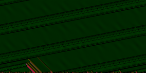
The following images show a 7.5 km long ring road divided into 1000 cells, on which vehicles drive from left to right. Starting at the bottom of the screen, the state of the road is shown second by second line by line upwards. A green point stands for a vehicle that last moved at speed 5, a red point means a stationary vehicle. Correspondingly, colors in between represent speeds of one to five cells per lap.
150 out of 1,000 street cells are occupied by a vehicle. The junk parameter p is p = 0.0. You can see how congestion - randomly existing at the beginning - dissolve.
At double the density (300 vehicles) and p = 0.15, the number of traffic jams increases dramatically.
The structure of the traffic jams changes in the VDR model. Here, too, there are 300 vehicles in the ring at p = 0.15 (for v> 0; for v = 0, p> 0.15)
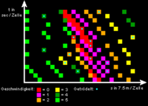
This graphic is an enlarged section of the illustration above with the junk parameter p = 0.15. Colored squares each mark a vehicle with its corresponding speed. Each line represents the occupation status of the same street. The occupancy status above each line (the street) shows the status in the following second.
Fundamental chart
A fundamental diagram is the plot of the flow over the density. Flow is the number of vehicles that pass a certain marking per lap (this can be a maximum of one on a single-lane road). Density is the proportion of the area of the road covered by vehicles (i.e. a maximum of one ). This plot (flow as y-coordinate, density as x-coordinate) is so characteristic of a certain parameter selection of a certain model that it is called a fundamental diagram.
Fundamental diagrams of the NaSch model
colour
model
Junk parameters p
Maximum speed v
deterministic
0.0
1
probabilistic
0.15
1
VDR
0.15
1
deterministic
0.0
5
probabilistic
0.15
5
VDR
0.15
5
The broken lines indicate how unstable the flow of traffic is at these points. In reality there is even a hysteresis effect : if the traffic slowly increases, you can still reach a fairly high flow at a certain density. At some point, when a driver overreacts when braking, this breaks down and drops to a significantly lower value. The traffic density must now decrease significantly in order to get back to the ascending branch of the fundamental diagram. Only then can an increase in density lead to an increased flow again. This effect has also already been observed in simulations .
Another point in which the real fundamental diagram differs from the fundamental diagrams of all the versions of the NaSch model discussed here is that the ascending branch of the fundamental diagram has a curvature in reality. The reason for this is that in reality the maximum speed of the vehicles is different. The curvature begins when the first vehicles reach their top speed. In order to implement this in the model, the NaSch model was expanded to include rules for multi-lane traffic and overtaking maneuvers. Without these rules, different maximum speeds would in principle always lead to traffic jams, as fast vehicles would collide with slow ones but would not be able to overtake.
In the deterministic case, the maximum is always at one density . For , the rules of movement for vehicles are identical to those for gaps (in the other direction). Therefore, the maximum is easily visible at the point where vehicles can move unhindered like gaps ( ).
Applications
The NaSch model was further developed for parallel computers by Kai Nagel in the United States and marketed under the name 'Transims'. Interestingly, the algorithm that not just on vector computers parallelize left and therefore Beowulf - Cluster are used. In the meantime, transims have been used to simulate all Swiss traffic in real time, with around 10 million vehicles.
K. Nagel, M. Schreckenberg: A cellular automaton model for freeway traffic . In: J. Phys. I France , 2, 1992, pp. 2221-2229.
K. Nagel: High-speed microsimulations of traffic flow . Dissertation, 1995.
K. Nagel: Particle hopping models and traffic flow theory . In: Physical Review E , 53, 1996, pp. 4655-4672.
M. Rickert, K. Nagel, M. Schreckenberg, A. Latour: Two Lane Traffic Simulations using Cellular Automats . In: Physica A , 231, 4, 1996, pp. 534-550.
A. Schadschneider, M. Schreckenberg: Car-oriented mean-field theory for traffic flow models . In: J. Phys. A: Math. Gen. , 30, 1997, pp. L69-L75.
K. Nagel, DE Wolf, P. Wagner, P. Simon: Two-lane traffic rules for cellular automata: A systematic approach . In: Physical Review E , 58, 1998, pp. 1425-1437.
A. Schadschneider, M. Schreckenberg: Garden of Eden states in traffic models . In: J. Phys. A: Math. Gen. , 31, 1998, pp. L225-L231.
D. Chowdhury, A. Pasupathy, S. Sinha: Distributions of time and distance headways in the Nagel-Schreckenberg model of vehicular traffic: effects of hindrances . In: European Physical Journal B , 5, 3, 1998, pp. 781-786.
R. Barlovic, L. Santen, A. Schadschneider, M. Schreckenberg: Metastable states in cellular automata for traffic flow . In: European Physical Journal B , 5, 3, 1998, pp. 793-800.
A. Schadschneider: Statistical Physics of Traffic Flow Models . In: Physica A , 285, 1-2, 2000, pp. 101-120.
C. Burstedde, K. Klauck, A. Schadschneider, J. Zittartz: Simulation of pedestrian dynamics using a two-dimensional cellular automaton . In: Physica A , 295, 3-4, 2001, pp. 507-525.
R. Barlovic, A. Schadschneider, M. Schreckenberg: Random walk theory of jamming in a cellular automaton model for traffic flow . In: Physica A , 294, 3-4, 2001, pp. 525-538.
W. Knospe, L. Santen, A. Schadschneider, M. Schreckenberg: A realistic two-lane traffic model for highway traffic . In: Journal of Physics A , 35, 2002, pp. 3369-3388.
B. Raney, A. Voellmy, N. Cetin, M. Vrtic, K. Nagel: Towards a Microscopic Traffic Simulation of All of Switzerland . In: Computational Science - ICCS 2002 , 2002, pp. 371-380.
A. Pottmeier, R. Barlovic, W. Knospe, A. Schadschneider, M. Schreckenberg: Localized defects in a cellular automaton model for traffic flow with phase separation . In: Physica A , 308, 1-4, 2002, pp. 471-482.
HK Lee, R. Barlovic, M. Schreckenberg, D. Kim: Mechanical Restriction versus Human Overreaction Triggering Congested Traffic States . In: Phys. Rev. Lett. , 92, 2004, p. 238702.