Cobb-Douglas function

Cobb-Douglas function of form . You can see the amount produced depending on the capital and labor input ${\displaystyle Y=0.1K^{1.5}L^{0.25}}$

In economics (especially in microeconomics ) and econometrics , the Cobb-Douglas function is a class of functions that is often used to formulate utility and production functions. If the Cobb-Douglas function under consideration meets specific requirements, it is more generally a neoclassical production function .

Historical background

The Cobb-Douglas function is based on knowledge that Johann Heinrich von Thünen gained in agriculture in the first half of the 19th century. With its per capita capital gains function

${\displaystyle p=c\cdot q^{n}}$

He developed the first indirectly formulated Cobb-Douglas production function with as a level parameter, and as yield or capital input per worker and as the substitution elasticity of capital. ${\displaystyle c}$ ${\displaystyle p}$ ${\displaystyle q}$ ${\displaystyle n}$

Two early works are often cited in the history of the Cobb-Douglas function: Coordination of the Laws of Distribution (1894) by Philip Wicksteed and Lectures (1901) by Knut Wicksell (or Ekonomisk Tidskrift , 1900). Despite these publications, it can be shown that Wicksell implicitly used its functional relationship as early as 1895 and explicitly used it from 1900.

The Swedish economist Knut Wicksell (1851–1926) succeeded in formulating the relationships between production factors and total production with an existing elasticity of substitution as a production function in the form known today.

Paul Howard Douglas

The American economist Paul Howard Douglas began in 1927 with a first formulation of the Cobb-Douglas production function. Using the example of the manufacturing industry in the USA between 1899 and 1922, Douglas empirically dealt with the question of the relationship between production there and the capital stock and the number of workers employed . In search of a functional description of this relationship - a so-called production function - he discussed with a colleague, the mathematician Charles Wiggins Cobb , who had previously used the function Wicksell and Wicksteed had already used ${\displaystyle Y}$ ${\displaystyle K}$ ${\displaystyle L}$

${\displaystyle Y=b\cdot L^{k}K^{1-k}}$

proposed.

In 1928 they estimated using the method of least squares for - the so-called production elasticity of labor - a value of ; the result was later replicated by the National Bureau of Economic Research with a value of approximately. ${\displaystyle k}$ ${\displaystyle 0{,}75}$ ${\displaystyle 0{,}741}$

definition

A Cobb-Douglas function is generally a function given by: ${\displaystyle z\colon \mathbb {R} _{+}^{n}\to \mathbb {R} _{+}}$

${\displaystyle z(x_{1},\dotsc ,x_{n})=\beta \cdot \prod _{i=1}^{n}x_{i}^{\alpha _{i}}=\beta \cdot x_{1}^{\alpha _{1}}\cdot \dotsc \cdot x_{n}^{\alpha _{n}}}$

with ; and for everyone . ${\displaystyle \beta >0}$ ${\displaystyle x_{i}>0}$ ${\displaystyle \alpha _{i}>0}$ ${\displaystyle i=1,\dotsc ,n}$

The level parameter causes the function to be scaled up or down, depending on the size. Thus, the level parameter can be viewed as a kind of efficiency parameter of the company or economy. In the literature, the level parameter is regularly omitted or it is set to one, since it becomes obsolete if the other factors are scaled accordingly. ${\displaystyle \beta }$

Another restriction is that the exponents just add up to one, that is, therefore

${\displaystyle \sum \nolimits _{i=1}^{n}\alpha _{i}=\alpha _{1}+\dotsb +\alpha _{n}=1}$.

This assumption guarantees constant returns to scale . In the case of production functions, constant economies of scale mean that an increased / decreased use of production factors leads to an increased / decreased production in the same proportion. A doubling of all factor inputs of the production factors thus leads to a doubling of the total production. With ordinal utility functions , the assumption of constant returns to scale is synonymous with homothety ; it induces linear angel curves .

Different uses

Amount produced depending on the capital and labor input

If the function is used as a production function, it is regularly referred to as (instead of ) to express that it shows the quantity of a good produced. They then stand for the amount of the production factor used , whereby there are production factors. For example, the two-factor Cobb-Douglas production function (sometimes simplified to with ) is often used , where the capital and labor input are used. ${\displaystyle Y}$ ${\displaystyle z}$ ${\displaystyle x_{i}}$ ${\displaystyle i}$ ${\displaystyle n}$ ${\displaystyle Y=\beta \cdot L^{\alpha _{1}}K^{\alpha _{2}}}$ ${\displaystyle Y=L^{\alpha }K^{1-\alpha }}$ ${\displaystyle 0<\alpha <1}$ ${\displaystyle K}$ ${\displaystyle L}$

When used as a utility function (usually ; from English utility for benefit) denotes the amount of goods consumed . For the two-goods case, the form is mostly used ; because of the monotonous transformability of ordinal utility functions, the factor would be obsolete anyway. Here, too, the exponents add up to one in order to preserve the property of constant returns to scale (which, as described above, is also justified by the transformability of the utility function). ${\displaystyle u}$ ${\displaystyle x_{i}}$ ${\displaystyle i}$ ${\displaystyle u(x_{1},x_{2})=x_{1}^{\alpha }\cdot x_{2}^{1-\alpha }}$ ${\displaystyle \beta }$

properties

Interpretation of elasticity

The central feature of functions of the Cobb-Douglas type is that the exponent of a direct interpretation are accessible, but it is at just about the elasticity of respect . For example, if you look at the Cobb-Douglas production function, it is the so-called production elasticity of the production factor - it indicates approximately by how many percent of total production increases if the amount of the factor used is increased by one percent. For example, assume the following Cobb-Douglas production function for an economy ${\displaystyle \alpha _{i}}$ ${\displaystyle z}$ ${\displaystyle x_{i}}$ ${\displaystyle \alpha _{i}}$ ${\displaystyle i}$ ${\displaystyle y}$ ${\displaystyle i}$

${\displaystyle Y(t)=T\cdot K(t)^{\alpha }L(t)^{1-\alpha }}$ With ${\displaystyle \alpha \in (0,1)}$

authoritative. At any point in time ( ), total production is produced in the economy using the production factors labor ( ) and capital ( ) with the help of a given technology level ( ). Then referred to here ${\displaystyle t}$ ${\displaystyle L}$ ${\displaystyle K}$ ${\displaystyle T}$

${\displaystyle \sigma _{K}\equiv {\frac {\partial Y}{\partial K}}{\frac {K}{Y}}={\frac {[\alpha \cdot T\cdot K(t)^{\alpha -1}L(t)^{1-\alpha }]\cdot K(t)}{T\cdot K(t)^{\alpha }L(t)^{1-\alpha }}}=\alpha }$

the production elasticity of capital, which for this production function corresponds to the exponent , which in turn represents the capital income ratio. Consequently, with an (infinitesimal) small increase in capital, total production increases by the capital income ratio. ${\displaystyle \alpha }$

The same applies to the production elasticity of labor

${\displaystyle \sigma _{L}\equiv {\frac {\partial Y}{\partial L}}{\frac {L}{Y}}={\frac {[(1-\alpha )\cdot T\cdot K(t)^{\alpha }L(t)^{-\alpha }]\cdot L(t)}{T\cdot K(t)^{\alpha }L(t)^{1-\alpha }}}=(1-\alpha )}$

that it corresponds to the exponent ( ), which in turn represents the wage income share. These results are mainly used in growth theory . ${\displaystyle 1-\alpha }$

Substitution elasticity

In a Cobb-Douglas production function, the elasticity of substitution - that is, the ratio of the relative change in the ratio of factor input to the relative change in the marginal rate of substitution - is always one. For the above The Cobb-Douglas production function therefore applies to the elasticity of substitution

${\displaystyle \sigma _{K,L}\equiv {\frac {\mathrm {d} \ln(K/L)}{\mathrm {d} \ln(Y_{L}/Y_{K})}}=1}$

Corresponding demand functions

Demand functions that are obtained from a Cobb-Douglas utility function have the property that households always spend a constant proportion of their income on goods . This application is an example of why the property mentioned in the previous section often makes it easier to use the function; the exponent can then be interpreted directly as the constant component sought. ${\displaystyle x_{i}}$ ${\displaystyle {\tfrac {a_{i}}{\sum \nolimits _{i=1}^{n}\alpha _{i}}}}$ ${\displaystyle \sum \nolimits _{i=1}^{n}\alpha _{i}=1}$

Returns to scale and elasticity of scale

The economies of scale are for constant (i.e. in the case of a production function, for example, that total production doubles if the input quantities of the production factors are doubled), for decreasing (a doubling of the input quantity of the production factors leads to less than a doubling of total production) and for increasing (a doubling of the input quantity of the production factors leads to more than a doubling of the total production). ${\displaystyle \sum \nolimits _{i=1}^{n}\alpha _{i}=1}$ ${\displaystyle \sum \nolimits _{i=1}^{n}\alpha _{i}<1}$ ${\displaystyle \sum \nolimits _{i=1}^{n}\alpha _{i}>1}$

The scale elasticity - that is the approximate change in production in percent as a result of a one percent increase in all factors of production - the sum of the exponents . ${\displaystyle \sum \nolimits _{i=1}^{n}\alpha _{i}}$

Homogeneity and (quasi) concavity

In general, it also applies that the Cobb-Douglas function is homogeneous in degree in the defined sense . Furthermore, it is quasi-concave for everyone ; concave if and even strictly concave if . ${\displaystyle \sum \nolimits _{i=1}^{n}\alpha _{i}}$ ${\displaystyle \alpha _{i}}$ ${\displaystyle \sum \nolimits _{i=1}^{n}\alpha _{i}\leq 1}$ ${\displaystyle \sum \nolimits _{i=1}^{n}\alpha _{i}<1}$

Strict essentiality

The Cobb-Douglas production function still has the property of strict essentiality d. This means that the output rate is 0 if nothing is used by a production factor. This property implies that the function always passes through the origin. Formally,

${\displaystyle z(x_{1},\dotsc ,x_{i-1},0,x_{i+1},\dotsc ,x_{n})=0\;\;\forall x_{i}}$.

For example, an economy whose production can be modeled with a Cobb-Douglas production function with the production factors labor and capital cannot generate any total production if one of the factors is not used.

Examples

Linear-homogeneous Cobb-Douglas production function

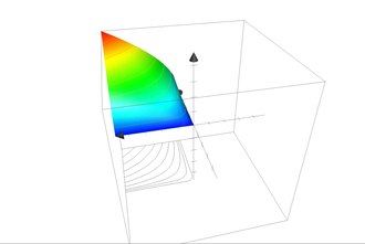
In the figure, a linear, homogeneous Cobb-Douglas production function is shown as a “production mountain range”. The area of ​​the mountain is made up of straight lines that emanate from the origin . If one production factor is kept constant and the other production factor is increased ( ceteris paribus analysis), then the total production also increases, but to an ever smaller extent, the partial marginal productivity of a factor decreases with increasing input of this factor. The partial marginal productivity is the slope of the production mountain range if one moves on it perpendicular to the axis of the constant production factor. ${\displaystyle (0{,}0{,}0)}$

If the economy moves along a “contour line”, the use of one production factor is substituted for that of the other . The law of the decreasing marginal rate of technical substitution applies .

The following three-dimensional representation shows a Cobb-Douglas production function of the form . The contour lines, which are in the form of indifference curves , can be represented by a horizontal section through the mountain of benefits and a subsequent projection onto the plane. ${\displaystyle z(x_{1},x_{2})=x_{1}^{1/2}\cdot x_{2}^{1/2}}$ ${\displaystyle x_{1}-x_{2}}$

Play media file

"Projection" of the contour lines into the plane (animation). ${\displaystyle x_{1}-x_{2}}$

Scope of the production function

The Cobb-Douglas production function is particularly useful for modeling larger economic systems (from larger companies to entire economies). Empirical studies of the German chemical industry between 1960 and 1975 gave, for example, the following estimate:

• Beiersdorf AG : ${\displaystyle \quad Y=e^{0,04t}L^{0,84}K^{0,39}}$

• BASF : ${\displaystyle \quad Y=e^{0,07t}L^{0,51}K^{0,49}}$

The regression coefficient has been replaced by a parameter that increases over time and shows technical progress. ${\displaystyle \beta }$ ${\displaystyle t}$

From the point of view of business administration , the Cobb-Douglas production function is too highly aggregated . In the case of very large companies, one can approximately assume that the factors labor and capital can be divided at will, but this is not the case for most companies. Arbitrary divisibility, however, is an implicit assumption of the Cobb-Douglas production function which leads to it being differentiable. Therefore, the Gutenberg production function was developed in business administration , which comes closer to operational practice.

Econometric model

The Cobb-Douglas function can easily be represented as an econometric model by a few transformations . Assume the following Cobb-Douglas function:

${\displaystyle Y_{t}=T\cdot K_{t}^{\alpha }L_{t}^{1-\alpha }}$ With ${\displaystyle \alpha \in (0,1)}$

The first step is to calculate the per capita version of the function for better handling:

${\displaystyle {\frac {Y_{t}}{L_{t}}}={\frac {T\cdot K_{t}^{\alpha }L_{t}^{1-\alpha }}{L_{t}}}=A\cdot \left({\frac {K_{t}}{L_{t}}}\right)^{\alpha }}$

In order to obtain a linear model, the function is linearized by logarithmizing:

${\displaystyle \ln \left({\frac {Y_{t}}{L_{t}}}\right)=\ln \left(A\cdot \left({\frac {K_{t}}{L_{t}}}\right)^{\alpha }\right)=\ln \left(A\right)+\alpha \cdot \ln \left({\frac {K_{t}}{L_{t}}}\right)}$

So we finally get the econometric model:

${\displaystyle y_{t}=\beta _{1}+x_{t2}\beta _{2}+\varepsilon _{t}}$ in which ${\displaystyle \beta _{1}=\ln \left(A\right),\;\beta _{2}=\alpha ,\;y_{t}=\ln \left({\frac {Y_{t}}{L_{t}}}\right),\;x_{t2}=\ln \left({\frac {K_{t}}{L_{t}}}\right)}$

The unknown parameters of this model can be estimated using single linear regression . The logarithmization shows that the error term follows a logarithmic normal distribution ( ). In general, an econometric model with the production factors I and the total production factor Y can be represented as follows: ${\displaystyle \varepsilon _{t}}$ ${\displaystyle \varepsilon _{t}\sim {\text{log-normal}}(\mu ,\sigma ^{2})}$

${\displaystyle \ln(Y_{t})=\beta _{1}+\sum _{k=2}^{K}\beta _{k}\ln(I_{tk})}$.

See also

• Leontief production function
• Solow model

literature

• Charles W. Cobb and Paul H. Douglas : A Theory of Production. In: The American Economic Review. 18, No. 1 (Supplement, Papers and Proceedings of the Fortieth Annual Meeting of the American Economic Association), 1928, pp. 139-165 ( JSTOR 1811556 ).
• Paul H. Douglas: The Cobb-Douglas Production Function Once Again: Its History, Its Testing, and Some New Empirical Values. In: Journal of Political Economy. 84, No. 5, 1976, pp. 903-916. [Overview of the history and different functional specifications in the literature.]
• Alfred Endres and Jörn Martiensen: Microeconomics. An integrated presentation of traditional and modern concepts in theory and practice. Kohlhammer, Stuttgart 2007, ISBN 978-3-17-019778-7 .
• Geoffrey A. Jehle and Philip J. Reny: Advanced Microeconomic Theory. 3rd ed. Financial Times / Prentice Hall, Harlow 2011, ISBN 978-0-273-73191-7 .
• Knut Sydsæter u. a .: Further mathematics for economic analysis. 2nd ed. Financial Times / Prentice Hall, Harlow 2008, ISBN 978-0-273-71328-9 .
• Knut Sydsæter, Arne Strøm and Peter Berck: Economists' mathematical manual. 4th edition. Springer, Berlin a. a. 2005, ISBN 978-3-540-26088-2 (also as an e-book: doi : 10.1007 / 3-540-28518-0 ).
• Johann Heinrich von Thünen : The isolated state in relation to agriculture and national economy. 3rd edition, edited by H. Schumacher-Zarchlin. Second part. II. Division. Berlin 1875.
• Hal Varian : Intermediate Microeconomics. A modern approach. 8th edition. WW Norton, New York and London 2010, ISBN 978-0-393-93424-3 .
• Hal Varian : Microeconomic Analysis. WW Norton, New York and London 1992, ISBN 0-393-95735-7 .
• Susanne Wied-Nebbeling and Helmut Schott: Fundamentals of microeconomics. Springer, Heidelberg a. a. 2007, ISBN 978-3-540-73868-8 .

Web links

• Interactive application for the Cobb-Douglas function

Individual evidence

1. ↑ Bo Sandlein in: John Cunningham Wood: Kurt Wicksell: Critical Assessments. P. 176.
2. ↑ Bo Sandlein: The early use of the Wicksell-Cobb-Douglas Function: A Comment on Weber. In: Journal and the History of Economic Thought. Volume 21, Number 2, 1999. p. 191.
3. ↑ ^{a b} See Peter H. Douglas: The Cobb-Douglas Production Function Once Again: Its History, Its Testing, and Some New Empirical Values. In: Journal of Political Economy. 84, No. 5, 1976, pp. 903-916 ( JSTOR 1830435 ), here p. 904; see also Wicksell-Cobb-Douglas production function - definition in the Gabler Wirtschaftslexikon.
4. ^ Charles W. Cobb and Paul H. Douglas: A Theory of Production. In: The American Economic Review. 18, No. 1 (Supplement, Papers and Proceedings of the Fortieth Annual Meeting of the American Economic Association), 1928, pp. 139-165 ( JSTOR 1811556 ).
5. ↑ The definition here follows, among others, Sydsæter u. a. 2008, p. 72; Wied-Nebbeling / Schott 2007, p. 121; Endres / Martiensen 2007, p. 227.
6. ↑ Isidro Soloaga: The Treatment of Non-essential Inputs in a Cobb-douglas Technology , p. 2
7. ↑ For example, Sydsaeter / Strøm / Berck 2005 S. 166th
8. ↑ only Varian 1992, p. 4; Jehle / Reny 2011, p. 68.
9. ↑ Sydsæter / Strøm / Berck 2005, p. 166.
10. ↑ Isidro Soloaga: The Treatment of Non-essential Inputs in a Cobb-douglas Technology , p. 2
11. ↑ Steven: Production Theory pp. 60–62
12. ^ Marno Verbeek: A Guide to Modern Econometrics , p. 94