Solow model

Graphical representation of the simple Solow model (Solow model without population growth and technical progress ) with per capita income on the vertical axis and per capita capital stock on the horizontal axis. You can see the equilibrium capital stock and the equilibrium per capita income . ${\displaystyle y}$ ${\displaystyle k^{*}}$ ${\displaystyle y^{*}}$

The Solow model , also known as the Solow-Swan model or Solow growth model , is a model developed in 1956 by Robert Merton Solow and Trevor Swan , which helps to explain the economic growth of an economy mathematically. It represents an exogenous growth model and forms a basis of the neoclassical growth theory . Due to its particularly attractive mathematical properties and mathematical simplicity, the Solow model proved to be a suitable starting point for a wide variety of extensions.

The Solow model explains growth as a process of accumulation of physical capital towards a long-term balance between investments and amortization , a so-called growth equilibrium or steady state ( English steady state ). At the core of the model is an aggregated neoclassical production function , which is mostly of the Cobb-Douglas type and which allows the macroeconomic model to “establish contact with the microeconomics ”. An economy at the beginning with little capital equipped is will save up in the model and thereby grow additional capital - initially high, with increasing capital accumulation until the long-term - then the low growth equilibrium is reached. In the long-term equilibrium, the growth rate of per capita output is zero. Further growth is only possible through ( exogenous ) technological progress that is not explained in the model , as this has the property that it overcomes the limitation of decreasing marginal yields.

History of origin

Solow and Swan independently developed similar versions of their growth model; Solow published his article in the Quarterly Journal of Economics in February 1956 , Swan's article appeared in November in Economic Record . While Swan's article also met with great professional reception at the beginning - the contribution was included several times in anthologies, and Swan was invited to various universities as a visiting professor - Solow's version of the model and in particular the graphic representation he selected prevailed in the long term. Solow later developed many implications and applications of this model and received the 1987 Nobel Prize in Economics for his contributions to growth theory.

The Solow-Swan model was a criticism and further development of the Harrod-Domar growth model that was prevalent at the time . Like the Solow model, the Harrod-Domar model also assumed a constant, exogenous savings rate. But the model was also based on a constant marginal productivity of capital and on a production function with little or no substitutability between labor and capital. The Harrod-Domar model allows several different growth equilibria: In one possible scenario capital grows without being used, in another, unemployment grows . A growth equilibrium results in which all available production factors are used only in one parameter constellation .

The model

Assumptions

In the Solow model, the economy is viewed as an aggregate unit (so to speak, as a single household) that carries out all production and consumption activities. Furthermore, the existence of a state is abstracted and it is assumed that there are no monetary effects, i. H. all goods prices are normalized to 1 . At any point in time, the economy possesses certain amounts of capital ( ), labor ( ) and technology ( ), which together produce according to a production function ( ), output ( ): ${\displaystyle (p\equiv 1)}$ ${\displaystyle t}$ ${\displaystyle K}$ ${\displaystyle L}$ ${\displaystyle T}$ ${\displaystyle F}$ ${\displaystyle Y}$

${\displaystyle Y_{t}=F(K_{t},T_{t}\cdot L_{t})}$

The product is called effective work . The production function is assumed to be neoclassical , i.e. it has the following four properties: ${\displaystyle T_{t}\cdot L_{t}}$ ${\displaystyle F}$

1. Essentiality of the factors of production. A production factor is called essential if, without its use, the output is always 0:

   ${\displaystyle F(K_{t}=0,T_{t}L_{t}>0)=0,\;\;F(K_{t}>0,T_{t}L_{t}=0)=0}$

2. Constant returns to scale or degree 1 homogeneity in effective work and capital. In economic terms, this means: An increased / decreased use of these production factors leads to an increased / decreased production in the same ratio:

   ${\displaystyle F(\lambda K_{t},\lambda T_{t}L_{t})=\lambda F(K_{t},T_{t}L_{t})}$

3. Positive and decreasing marginal yields:
   
   The marginal returns on capital and effective labor are positive, but decrease as the factor increases. For example, if more effective labor is used, production will increase, but it will rise less if much effective labor is already being used. Mathematically this means that the first partial derivatives of the production function according to effective labor and capital are positive, but the respective second derivatives are negative:

   ${\displaystyle {\frac {\partial F}{\partial K_{t}}}>0,\;\;{\frac {\partial ^{2}F}{\partial K_{t}^{2}}}<0}$

   ${\displaystyle {\frac {\partial F}{\partial (T_{t}L_{t})}}>0,\;\;{\frac {\partial ^{2}F}{\partial (T_{t}L_{t})^{2}}}<0}$

4. The so-called Inada conditions must be met, i. This means that the marginal product of every factor of production converges towards infinity, if one only lets the respective factor input tend towards zero. If, on the other hand, the respective factor input is allowed to tend towards infinity, the marginal product of the factor converges towards zero:

   ${\displaystyle \lim _{K_{t}\to 0}{\frac {\partial F}{\partial K_{t}}}=\infty \quad {\textrm {und}}\quad \lim _{K_{t}\to \infty }{\frac {\partial F}{\partial K_{t}}}=0}$

   ${\displaystyle \lim _{L_{t}\to 0}{\frac {\partial F}{\partial (T_{t}L_{t})}}=\infty \quad {\textrm {und}}\quad \lim _{L_{t}\to \infty }{\frac {\partial F}{\partial (T_{t}L_{t})}}=0}$

In economic terms, this means that given the technology in an economy, the output cannot be increased at will by increasing the labor input (or capital input). Thus a positive growth rate of income in the case of a neoclassical production function without technical progress is not possible in the long term if the Inada conditions apply.

In its simplest form, the Solow model also relates to a closed economy with no state activity . Income and production must correspond in such an economy, the production can therefore either be used for consumption or for investments (output use equation):

${\displaystyle Y_{t}=C_{t}+I_{t}}$

In addition, gross investments are exactly what the economy is saving ex post : (see also Investment and Saving ). In a closed economy is thus . The saving behavior of the economy is modeled by a constant savings rate ( ):, where is between 0 and 1. The economy therefore saves a certain percentage of the total production in each period. This savings rate , which is constant over time , is assumed to be an exogenous parameter that is not determined in the model. The results summarized apply: ${\displaystyle S_{t}\equiv I_{t}}$ ${\displaystyle S_{t}=Y_{t}-C_{t}}$ ${\displaystyle s=\mathrm {const.} }$ ${\displaystyle S_{t}=s\cdot Y_{t}}$ ${\displaystyle s}$ ${\displaystyle s}$

Approximate equality and constancy of savings and investment rates.

${\displaystyle Y_{t}=C_{t}+I_{t}=C_{t}+S_{t}=C_{t}+sY_{t}}$ With ${\displaystyle s\in [0,1]}$

Two further assumptions concern capital and labor: With regard to capital, it is assumed that in each period a certain percentage of the existing capital becomes unusable (depreciation), while the working population grows exponentially at a constant rate of growth . Furthermore, it is assumed that the savings rate corresponds to the investment rate due to the assumed equality of saving and investment . However, this is not a restrictive assumption, since in reality there is an approximate equality of the two quotas over time. ${\displaystyle \delta }$ ${\displaystyle n}$ ${\displaystyle s}$ ${\displaystyle \gamma }$

The growth process

→ Main article : Neoclassical theory

For the analysis of economies with growing populations and for better comparability of economies of different sizes, the model sizes are not expressed in absolute terms, but per capita, with lowercase letters being used for per capita sizes. One defines accordingly:

${\displaystyle y_{t}\equiv {\frac {Y_{t}}{L}}={\frac {F(K_{t},T_{t}L)}{L}}=F\left({\frac {K_{t}}{L}},T_{t}\right)}$,

where the last equation follows from the assumption of constant returns to scale .

Assuming a constant technology , the per capita production function can then be defined with per capita capital as ${\displaystyle T_{t}}$ ${\displaystyle k_{t}\equiv K_{t}/L}$

${\displaystyle f(k_{t})\equiv F\left({\frac {K_{t}}{L}},T_{t}\right)}$.

For each per capita capital stock , this indicates how much output is produced per capita. The per capita capital stock is therefore decisive for the development of per capita income . ${\displaystyle k_{t}}$

Its development is determined by three factors:

1. In each period the economy saves part of its per capita income: ${\displaystyle sy_{t}=sf(k_{t})}$
2. In every period a part of the per capita capital stock becomes : unusable ${\displaystyle \delta \in (0,1)}$ ${\displaystyle k}$ ${\displaystyle -\delta k}$
3. In each period, the population grows exponentially at an exogenous rate , so more workers need to be capitalized to keep per capita capital constant: ${\displaystyle n}$ ${\displaystyle L(t)=L(0)e^{nt}}$

The change in the per capita capital stock in each period is thus given as

Fundamental equation of motion of the Solow model with population growth:

${\displaystyle {\dot {k}}_{t}=\color {Green}sf(k_{t})-\color {Red}(n+\delta )k_{t}}$

• ${\displaystyle {\dot {k}}_{t}}$: Change in capital intensity over time
• ${\displaystyle sf(k_{t})}$: Gross investment per capita
• ${\displaystyle (n+\delta )k_{t}}$: Extended depreciation per capita
• ${\displaystyle sf(k_{t})-(n+\delta )k_{t}}$: Net investment per capita

If is positive, the per capita capital stock and with it the per capita income grows. If it is negative, then per capita capital and production shrink. Formally this means: ${\displaystyle {\dot {k}}_{t}}$ ${\displaystyle {\dot {k}}_{t}}$

${\displaystyle sf(k_{t})>(n+\delta )k_{t}\Rightarrow {\dot {k}}_{t}>0}$ (Capital intensity and per capita income grow)

${\displaystyle sf(k_{t})<(n+\delta )k_{t}\Rightarrow {\dot {k}}_{t}<0}$ (Capital intensity and per capita income shrink)

In the long-term equilibrium - the growth equilibrium level of the economy - it must be the case that the investments correspond exactly to the depreciation (taking into account population growth ) of the capital model, i. That is, the capital stock per capita is constant over time ( ): ${\displaystyle {\dot {k}}=0}$

${\displaystyle sf(k_{t})-(n+\delta )k_{t}=0\Leftrightarrow sf(k_{t}^{*})=(n+\delta )k_{t}^{*}}$

The per capita capital stock that satisfies this equation is the growth equilibrium capital stock ( ) of the economy. The above-mentioned assumptions about the production function (constant returns to scale, positive, decreasing marginal returns and the Inada conditions) guarantee the existence of a clear growth equilibrium. ${\displaystyle k_{t}}$ ${\displaystyle k_{t}^{*}}$

Fig. 1. Graphic representation of the Solow model with population growth: Regardless of the starting point, the capital intensity converges to the equilibrium capital intensity.

This can be shown graphically in a diagram with per capita capital on the horizontal and per capita income on the vertical axis: according to the assumptions, it is a concave function, as is the economic saving function . The curve is a straight line, which indicates how much must be saved to hold on to the per capita capital stock just constant and is therefore also known as investment demand line ( English requirement line designated). The intersection between the savings function and the investment requirement line determines the long-term equilibrium level (growth equilibrium) of the capital stock, in which just enough is saved that the capital stock remains constant despite depreciation and population growth. When this capital stock is reached, the rate of growth is zero and per capita output, income and capital are constant over time. ${\displaystyle f(k_{t})}$ ${\displaystyle sf(k_{t})}$ ${\displaystyle (n+\delta )k_{t}}$

If per capita capital is below the long-term equilibrium level, the economy will grow and eventually reach long-term equilibrium asymptotically. The growth rate continues to decrease with increasing capital stock - an implication of the assumption that the marginal returns on capital decrease. The Solow model thus predicts that, ceteris paribus , economies with a lower per capita capital stock will grow faster than those with a high capital endowment.

Convergence to equilibrium

Figure 2. Graphical representation of the change in the capital stock per capita over time. A - Chart ${\displaystyle t}$ ${\displaystyle {\dot {k}}_{t}-k_{t}}$

In the area where the investments ( ) are greater than the depreciation ( ), the net investments are positive and thus the capital intensity increases over time . In contrast to this, the net investments in the area in which the investments are smaller than the depreciation are negative and thus the capital intensity decreases over time . As a result, the system is globally stable ; i.e., for any initial value ( ), the economy converges to the growth equilibrium ( ) (global stability): ${\displaystyle sf(k_{t})}$ ${\displaystyle \delta k_{t}}$ ${\displaystyle {\dot {k}}_{t}>0}$ ${\displaystyle {\dot {k}}_{t}<0}$ ${\displaystyle k(0)>0}$ ${\displaystyle k^{*}}$

${\displaystyle {\dot {k}}_{t}>0\;\;\forall \;\;k_{t}<k^{*}}$

${\displaystyle {\dot {k}}_{t}<0\;\;\forall \;\;k_{t}>k^{*}}$

Changes in exogenous parameters

The long-term growth equilibrium capital stock ( ) is determined by, as stated above ${\displaystyle k^{*}}$

${\displaystyle sf(k_{t}^{*})=(\delta +n)k_{t}^{*}}$.

The savings rate , the depreciation rate and the population growth are viewed as exogenous parameters that are not determined in the model. However, changes in these parameters have an impact on the long-term equilibrium of the economy. ${\displaystyle s}$ ${\displaystyle \delta }$ ${\displaystyle n}$

Population growth and depreciation

Fig. 3. Effect of a higher rate of population growth ( ) on long-term equilibrium. ${\displaystyle n_{1}}$

Faster population growth (larger ) or larger depreciation (larger ) have the same effects on the long-term equilibrium level in the model: They increase the slope of the investment requirement line and thereby decrease per capita capital stock and income: in each period more workers have to be provided with capital (or more capital must be replaced) so that less per capita capital is formed with the same savings behavior and the same production technology. Fig. 3 graphically shows how the long-term equilibrium reacts to increased population growth: the black savings function line remains unchanged, the investment requirement line with a slope (red) rotates around the origin. The new long-term equilibrium results from the intersection of the changed investment requirement line with the savings function and is characterized by a lower per capita capital and income than the previous equilibrium . Since the new investment requirement line for capital stock is higher than , too little capital is saved - the economy is shrinking ( ). This process continues until the new equilibrium level in point (intersection of the new investment requirement line with the savings curve:) is reached. In the new equilibrium there is an equally weighted lower per capita capital stock and a lower equilibrium per capita output level is realized. ${\displaystyle n}$ ${\displaystyle \delta }$ ${\displaystyle (n+\delta )}$ ${\displaystyle \mathrm {B} }$ ${\displaystyle \mathrm {A} }$ ${\displaystyle k_{0}}$ ${\displaystyle sy_{0}}$ ${\displaystyle {\dot {k}}_{t}<0}$ ${\displaystyle \mathrm {B} }$ ${\displaystyle (n_{1}+\delta )k=sy}$ ${\displaystyle \mathrm {B} }$ ${\displaystyle k_{1}}$ ${\displaystyle y_{1}}$

Savings rate and the golden rule of accumulation

Fig. 4. Effect of a higher savings rate ( ) on the long-term equilibrium. ${\displaystyle s_{1}}$

An increase in the savings rate pushes the economy's savings curve upwards, which leads to an increase in the growth equilibrium per capita capital stock and thus per capita income as well. Fig. 4 illustrates this graphically: The increase in the savings rate shifts the savings function from its original position (black) upwards, while the investment requirement line (red) remains unchanged. The new equilibrium results from the intersection of the investment requirement line with the new savings function and has a larger capital stock and higher income per capita. ${\displaystyle \mathrm {B} }$

The effect of such an increase on consumption is not clear: on the one hand, more is produced in the long-term equilibrium, on the other hand, with a higher savings rate, per capita consumption is lower. Graphically, per capita consumption for a given per capita capital corresponds to the vertical distance between the production function and the saving function for the same per capita capital; In Fig. 4 this is the vertical distance between the red and green lines. This shows why the effect on consumption is fundamentally indeterminate: Although the new equilibrium shows higher production per capita in points, the new savings function is also closer to the production function. ${\displaystyle (1-s)y}$ ${\displaystyle \mathrm {B} }$

The golden rule of accumulation describes the savings rate in an economy that maximizes steady-state consumption:

${\displaystyle s^{\mathrm {gold} }\equiv {\underset {s}{\operatorname {arg\,max} }}\left\lbrace \color {Green}f(k^{*}(s))-\color {Red}(n+\delta )k^{*}(s)\right\rbrace }$.

Fig. 5. This graph shows how the capital stock and the associated savings rate maximize the economy's long-term equilibrium consumption . The maximum is . ${\displaystyle k^{\mathrm {gold} }}$ ${\displaystyle s^{\mathrm {gold} }}$ ${\displaystyle c^{*}}$ ${\displaystyle c^{\mathrm {gold} }}$

In long-term equilibrium , the following must apply to every savings rate . At the same time, the consumption level associated with the equilibrium is given by . For this reason, balanced consumption can be described as a function of the savings rate: ${\displaystyle s}$ ${\displaystyle k^{*}}$ ${\displaystyle sf(k^{*})=(n+\delta )k^{*}}$ ${\displaystyle c^{*}(s)=(1-s)f(k^{*})}$

${\displaystyle c^{*}(s)=f(k^{*}(s))-(n+\delta )k^{*}(s)}$

This can then be maximized via and results in the first-order condition ( necessary condition ): ${\displaystyle s}$

${\displaystyle {\frac {\partial c^{*}(s)}{\partial s}}=[f'(k^{*}(s))-n-\delta ]{\frac {\mathrm {d} k^{*}(s)}{\mathrm {d} s}}\;{\overset {\mathrm {!} }{=}}\;0}$,

where , so that the condition can be simplified to or (net marginal product of capital equals the rate of population growth). The capital stock that satisfies this equation and the associated savings rate maximize the economy's long-term equilibrium consumption (see Fig. 5 ). Although the savings rate found in this way maximizes equilibrium consumption, it is not clear whether this is desirable from an economy's point of view. For an economy that is also in equilibrium, an increase in the savings rate to a higher level of consumption in the long term means, but only when the new equilibrium is reached. ${\displaystyle \mathrm {d} k^{*}/\mathrm {d} s>0}$ ${\displaystyle f'(k^{*})=(n+\delta )}$ ${\displaystyle {\text{GPK}}-\delta =n}$ ${\displaystyle k^{\mathrm {gold} }}$ ${\displaystyle s^{\mathrm {gold} }}$ ${\displaystyle s<s^{\mathrm {gold} }}$ ${\displaystyle s^{\mathrm {gold} }}$

In the first periods after the increase in the savings rate, consumption would initially decrease (since the savings rate is increased, but not enough capital has yet been formed for the new growth equilibrium and as a result, production is still low compared to the new growth equilibrium). Depending on how much weight the economy puts on current versus future consumption, it might not be desirable to increase the savings rate today ( short term ) in order to achieve a new equilibrium with higher consumption in the long term. The case is different if the current savings rate is. In this case, a balance with higher consumption could be achieved by reducing the savings rate, i.e. consuming more. The economy would then consume more and more in the new equilibrium and also in the previous periods. A situation with is therefore called dynamically inefficient . ${\displaystyle s>s^{\mathrm {gold} }}$ ${\displaystyle s>s^{\mathrm {gold} }}$

Fig. 6 and Fig. 7 graphically show how different changes in the savings rate can affect. In Fig. 6 , the savings rate increases from an original, dynamically efficient equilibrium. The increase leads to positive capital growth and thus to increasing capital and income per capita. Capital growth decreases with increasing capital accumulation and approaches zero asymptotically, the economy reaches a new equilibrium with higher capital, income and consumption per capita. At the beginning of the process, however, this higher level in the long term has to be “bought” with lower consumption. Whether such a change in the savings rate is desirable from the point of view of the national economy depends on how the early consumption loss is assessed against the later consumption gain. In Fig. 7 , the savings rate is reduced based on a dynamically inefficient, i.e. excessively high, savings rate. The reduction leads to negative capital growth and thus to falling capital and income per capita. The capital contraction decreases with increasing capital accumulation and tends asymptotically towards zero, the economy reaches a new equilibrium with lower capital and income per capita. However, long-term per capita consumption is higher as less is saved. The main difference to the dynamically efficient situation is that consumption is not only higher in the long term, but also in every period from the increase. By lowering the savings rate, the economy can not only consume more in the long term, but also immediately. Regardless of the assessment of early versus later consumption, with a savings rate above the “golden” savings rate, a reduction in the savings rate is definitely desirable from the point of view of the economy.

• 

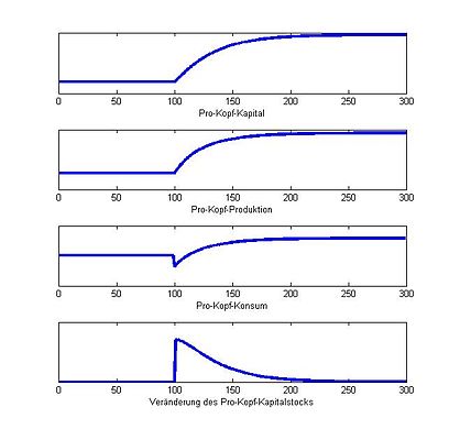
  Fig. 6. Increase in the savings rate based on a dynamically efficient situation. The specified values ​​are shown on the respective vertical axis, the horizontal axis shows the time. The change in the savings rate occurs over a period of time . ${\displaystyle 100}$

• 

  Fig. 7. Reduction of the savings rate based on a dynamically inefficient situation. The specified values ​​are shown on the respective vertical axis, the horizontal axis shows the time. The change in the savings rate occurs over a period of time . ${\displaystyle 100}$

→ Main article : Golden rule of accumulation

Technological progress

Technological progress shifts the production function and thus also the savings function up in the diagram; the new intersection with the investment requirement line is thus at a higher per capita capital and income level. Technological progress can therefore lead to growth even in long-term equilibrium. ${\displaystyle k-f(k)}$

With technological advances multiplying the labor production factor and the assumptions presented in Section 1.1, the production function can be divided by the factor . Instead of the previously used per capita production, this results in production per effective unit of work (per efficiency unit) depending on the capital stock per effective unit of work: ${\displaystyle Y_{t}=F(K_{t},T_{t}L_{t})}$ ${\displaystyle T_{t}\cdot L_{t}}$

${\displaystyle {\tilde {y}}_{t}\equiv {\frac {Y_{t}}{T_{t}L_{t}}}=F\left({\frac {K_{t}}{T_{t}L_{t}}},1\right)\equiv f\left({\tilde {k}}_{t}\right)}$

As before, the investment requirement per effective unit of work results from the depreciation rate and population growth; Now, however, the increased labor productivity as a result of technological progress must also be compensated: Technological progress leads to an increase in the effective units of work (the product increases), so the capital per effective unit of work falls, ceteris paribus. Assuming exponential technology growth with a growth rate, the investment requirement line for capital per effective unit of work results as . The equation of motion for the capital per effective unit of work is thus: ${\displaystyle T_{t}\cdot L_{t}}$ ${\displaystyle g}$ ${\displaystyle (\delta +n+g){\tilde {k}}_{t}}$

Fundamental equation of motion of the Solow model with population growth and technological progress:

${\displaystyle {\dot {\tilde {k}}}_{t}=\color {Green}sf({\tilde {k}}_{t})-\color {Red}(\delta +n+g){\tilde {k}}_{t}}$

Long-term equilibrium is reached when the capital stock per effective unit of work is constant, i.e. when:

${\displaystyle sf({\tilde {k}}_{t})=(\delta +n+g){\tilde {k}}_{t}}$

The capital stock and thus also the income per effective unit of work do not grow in the long-term equilibrium. However, the per capita income is given by

${\displaystyle y_{t}\equiv Y_{t}/L_{t}=[Y/T_{t}L_{t}]\cdot T_{t}={\tilde {y}}_{t}T_{t}}$.

It grows at the same rate as the technology of the economy . A growth in per capita sizes in long-term equilibrium is therefore possible, but only due to exogenous technological progress. ${\displaystyle g}$

Example: Solow model with Cobb-Douglas production function

A possible production function that fulfills the assumptions presented above is the following Cobb-Douglas function :

${\displaystyle Y_{t}=T\cdot K_{t}^{\alpha }L_{t}^{1-\alpha }}$ With ${\displaystyle \alpha \in (0,1)}$

At any point in time, output is produced in the economy using the production factors labor and capital with the help of a given level of technology . The restriction on the production elasticity of capital is that it must lie between and . The same restriction follows for the elasticity of production of labor . After dividing the production function by the size of the population, the per capita version results . The equation of motion of the per capita capital stock (capital accumulation equation) is then given by ${\displaystyle L}$ ${\displaystyle K}$ ${\displaystyle T}$ ${\displaystyle 0}$ ${\displaystyle 1}$ ${\displaystyle (1-\alpha )}$ ${\displaystyle y_{t}=T\cdot k_{t}^{\alpha }}$

${\displaystyle {\dot {k}}_{t}=\color {Green}sTk_{t}^{\alpha }-\color {Red}(n+\delta )k_{t}}$.

The long-term equilibrium is when this change is zero and consequently

${\displaystyle sTk_{t}^{\alpha }=(\delta +n)k_{t}\Leftrightarrow k_{t}^{1-\alpha }={\frac {sT}{\delta +n}}}$,

and so then applies to the equilibrium capital intensity

${\displaystyle k^{*}=\left({\frac {sT}{\delta +n}}\right)^{\frac {1}{1-\alpha }}}$.

For the equilibrium per capita income thus follows

${\displaystyle y^{*}=T^{\frac {1}{1-\alpha }}\left({\frac {s}{\delta +n}}\right)^{\frac {\alpha }{1-\alpha }}}$

and for per capita consumption in the stationary state ( ) thus applies ${\displaystyle c^{*}=(1-s)y^{*}}$

${\displaystyle c^{*}=(1-s)T^{\frac {1}{1-\alpha }}\left({\frac {s}{\delta +n}}\right)^{\frac {\alpha }{1-\alpha }}}$.

Using the equation of , it can be seen that differences in , i.e. differences in the level of technology, the savings rate, the depreciation rate, the growth rate of the population and the production elasticity of capital can explain the differences in per capita income between countries (at least in part). Because of a higher savings rate and a higher level of technology lead to a higher equilibrium capital stock, while faster population growth and a higher depreciation rate lead to a lower equilibrium. ${\displaystyle y^{*}}$ ${\displaystyle T,s,\delta ,n,\alpha }$ ${\displaystyle \alpha <1}$

Furthermore, it can be shown that the above production function fulfills the assumptions mentioned under 1.1:

1. Constant returns to scale:

The property of constant returns to scale is fulfilled:

${\displaystyle {\begin{aligned}F(\lambda K_{t},\lambda L_{t})&=T\cdot (\lambda K_{t})^{\alpha }(\lambda L_{t})^{1-\alpha }\\&=T\cdot \lambda ^{\alpha }K_{t}^{\alpha }\lambda ^{1-\alpha }L_{t}^{1-\alpha }\\&=\lambda T\cdot K_{t}^{\alpha }L_{t}^{1-\alpha }=\lambda F(K_{t},L_{t}).\end{aligned}}}$

2. Positive and decreasing marginal yields:

The marginal products of capital and labor are positive:

${\displaystyle {\text{GPA}}\equiv {\frac {\partial F(K_{t},L_{t})}{\partial L_{t}}}=(1-\alpha )\cdot T\cdot K_{t}^{\alpha }L_{t}^{-\alpha }>0}$

${\displaystyle {\text{GPK}}\equiv {\frac {\partial F(K_{t},L_{t})}{\partial K_{t}}}=\alpha \cdot T\cdot K_{t}^{\alpha -1}L_{t}^{1-\alpha }>0}$

Since the partial derivatives can only be positive due to the restriction , you can see that the output rises when the respective input factors increase. The partial derivatives of the 2nd order give: ${\displaystyle \alpha \in (0,1)}$

${\displaystyle {\frac {\partial ^{2}F(K_{t},L_{t})}{\partial L_{t}^{2}}}=-\alpha (1-\alpha )\cdot T\cdot K_{t}^{\alpha }L_{t}^{-\alpha -1}<0}$

${\displaystyle {\frac {\partial ^{2}F(K_{t},L_{t})}{\partial K_{t}^{2}}}=\alpha (\alpha -1)\cdot T\cdot K_{t}^{\alpha -2}L_{t}^{-\alpha }<0}$

They will be negative for all inputs, so the growth rates will fall (there are decreasing marginal yields). So you could say that if the input rises, the output rises below proportionally .

3. The Inada conditions are met:

${\displaystyle \lim _{K_{t}\to 0}{\frac {\partial F(K_{t},L_{t})}{\partial K_{t}}}=\infty \quad {\textrm {und}}\quad \lim _{K_{t}\to \infty }{\frac {\partial F(K_{t},L_{t})}{\partial K_{t}}}=0}$

${\displaystyle \lim _{L_{t}\to 0}{\frac {\partial F(K_{t},L_{t})}{\partial L_{t}}}=\infty \quad {\textrm {und}}\quad \lim _{L_{t}\to \infty }{\frac {\partial F(K_{t},L_{t})}{\partial L_{t}}}=0}$

The Inada conditions imply (together with the above assumptions) that for exactly a stable equilibrium with exist, in which therefore the capital stock is constant over time. ${\displaystyle k_{t}\in (0;\infty )}$ ${\displaystyle k^{*}}$ ${\displaystyle {\dot {k}}=0}$

Different savings rates

In the following, a comparative static analysis is used to show how the savings rate determines the per capita income of the respective country. For the comparison, two countries are used that differ greatly in their savings rate. B. Korea and Uganda . In the case of Korea, one assumes an estimated savings rate of and in the case of Uganda an estimated savings rate of . Furthermore, a capital income ratio of is assumed (empirically, the capital income ratio in most countries is around ). To show the effects on per capita income if the two countries differ only in the savings rate, the equilibrium per capita incomes of the two countries are put in relation ( comparative statics ): ${\displaystyle s_{1}=\color {BrickRed}0{,}2}$ ${\displaystyle s_{2}=\color {BrickRed}0{,}05}$ ${\displaystyle (\alpha )}$ ${\displaystyle \color {BrickRed}1/3}$ ${\displaystyle \color {BrickRed}1/3}$

${\displaystyle {\frac {y_{1}^{*}}{y_{2}^{*}}}={\frac {T^{\frac {1}{1-\alpha }}\left({\frac {s_{1}}{\delta +n}}\right)^{\frac {\alpha }{1-\alpha }}}{T^{\frac {1}{1-\alpha }}\left({\frac {s_{2}}{\delta +n}}\right)^{\frac {\alpha }{1-\alpha }}}}={\frac {\left({\frac {s_{1}}{\delta +n}}\right)^{\frac {\alpha }{1-\alpha }}}{\left({\frac {s_{2}}{\delta +n}}\right)^{\frac {\alpha }{1-\alpha }}}}=\left({\frac {s_{1}}{s_{2}}}\right)^{\frac {\alpha }{1-\alpha }}}$

For the above example this results in:

${\displaystyle {\frac {y_{1}^{*}}{y_{2}^{*}}}=\left({\frac {\color {BrickRed}0{,}2}{\color {BrickRed}0{,}05}}\right)^{\frac {\color {BrickRed}1}{\color {BrickRed}2}}=\color {BrickRed}2}$

So, according to the Solow model, Korea is twice as rich as Uganda. In fact, Korea is about 13 times as rich. As a result, differences in income can only partly be explained by the Solow model.

Empirical Applications

Growth accounting

Closely related to the Solow model is the so-called growth accounting ( English growth accounting ) that of Moses Abramovitz was pushed and Robert Solow. It examines what proportion of economic growth can be explained by capital, labor and other factors. For a general production function of the form it can be shown that the growth of the total production can be divided by means ${\displaystyle Y_{t}=F(K_{t},L_{t},T_{t})}$

${\displaystyle {\widehat {Y_{t}}}-{\widehat {L_{t}}}=\alpha _{K_{t}}\left({\widehat {K_{t}}}-{\widehat {L_{t}}}\right)+R_{t}}$,

where indicates the elasticity of production in relation to capital. In this way, economic growth per capita can be divided into per capita growth due to per capita capital accumulation and another additive term , the so-called Solow residual . This is sometimes interpreted as the contribution of technological progress to growth, but is actually a collective term for all factors that lead to economic growth and are not already covered by capital accumulation. ${\displaystyle \alpha _{K_{t}}}$ ${\displaystyle R_{t}}$

convergence

If the economy is still below long-term equilibrium and growing, the lower the per capita capital stock is, the higher its growth rate. According to the Solow model, an economy with originally little per capita capital will initially have very high growth rates, which then decrease with increasing capital accumulation and finally tend towards 0. For two economies with the same technology and the same exogenous parameters (depreciation rate, savings rate, population growth) and thus the same long-term equilibrium, but different original capital resources, the model predicts that the originally poorer economy will grow faster and thus "catch up" with the originally richer economy becomes ( catch-up effect ). This process is also known as " convergence". ${\displaystyle \beta }$

Absolute convergence

The absolute convergence states that two countries with different GDP and capital per capita starting levels, but with the same levels in the savings rate, depreciation rate, population growth rate and the rate of technical progress will converge in the long term to the same level of capital stock and GDP per capita ( Countries with initially lower income levels grow faster due to decreasing marginal yields). In summary, countries grow faster the further they are from their specific long-term equilibrium. A prediction of the model would not be that poor countries grow faster than rich ones, but that among “similar” countries (countries with similar parameters) the originally poorer countries show higher growth rates. Indeed, there is a negative correlation between their per capita income in 1960 and the average annual growth rate between 1960 and 2000 among OECD countries . An even more pronounced negative correlation exists between the per capita income of the US states in 1880 and their annual growth rates between 1880 and 2000. However, the Solow model does not predict absolute convergence , where all poor countries equally catch up and converge towards the same long-term equilibrium. The hypothesis of the Solow model is instead of conditional convergence.

Conditional convergence

In the Solow model, economies converge to different steady-state states, provided that these have differences in the model parameters. If countries differ in total factor productivity, the savings rate or the depreciation rate, they consequently differ in their long-term equilibrium (different regional stationary states). Often the conditional convergence is empirical instead of the absolute.

Empirical results

Another test for convergence was carried out by N. Gregory Mankiw , David Romer and David N. Weil in 1992. Based on a sample of 98 countries, they showed that there was no correlation between per capita income in 1960 and the growth rate between 1960 and 1985, i.e. no absolute convergence. If, however, statistical controls are used for the investment rate and population growth, a negative effect of the original income level becomes apparent, which supports the hypothesis of conditional convergence. The standard Solow model, however, overestimates the speed of convergence, and the actual catching up is slower than predicted by the model. Mankiw, Romer and Weil were able to show, however, that a Solow model expanded to include human capital as the third production factor predicts roughly the same speed of convergence that is also visible in the data. In this extended model, the production function also has the human capital factor and is: ${\displaystyle H}$

${\displaystyle Y_{t}=K_{t}^{\alpha }H_{t}^{\beta }(T_{t}L_{t})^{1-\alpha -\beta }}$with . ${\displaystyle \alpha +\beta <1}$

The human capital per effective unit of work develops according to an equation of motion similar to that for the capital per effective unit of work: ${\displaystyle {\tilde {h_{t}}}}$

${\displaystyle {\dot {\tilde {h}}}=\color {Green}s_{h}{\tilde {y_{t}}}-\color {Red}(n+g+\delta ){\tilde {h_{t}}}}$,

where the (also exogenous) investment rate for human capital denotes. In the equilibrium of growth, capital and human capital per effective unit of work are then constant. ${\displaystyle s_{h}}$

International and historical income differences

According to the Solow model, there are two possible reasons for per capita income differences between economies: different per capita capital stocks and different labor productivity. In fact, however, the per capita capital stock cannot explain the large income gaps between rich and poor countries today or between developed countries then and now. The per capita income of industrialized countries is now about ten times greater than a century before; the natural logarithms of per capita income today and years ago therefore differ by . With the definition of the elasticity of per capita income in relation to per capita capital,, follows . With it follows that the difference in per capita capital stock ${\displaystyle 100}$ ${\displaystyle \ln(10)}$ ${\displaystyle \alpha _{K}}$ ${\displaystyle \alpha _{K}\equiv \mathrm {d} \log(y)/\mathrm {d} \log(k)}$ ${\displaystyle \mathrm {d} \log(k)=\mathrm {d} \log(y)/\alpha _{K}}$ ${\displaystyle \mathrm {d} \log(y)=\ln(10)}$

${\displaystyle \operatorname {exp} \left({\frac {\ln(10)}{\alpha _{K}}}\right)=10^{1/\alpha _{K}}}$

must be. Empirical studies suggest that this is around a third. If the per capita capital would be the only source for per capita income differences, the per capita capital would have in recent years say by about a factor grew to be, a growth of per capita income by a factor of about to explain. In fact, per capita capital has only grown by about one factor . The growth in per capita capital can not explain the extent of economic growth over the past few years. ${\displaystyle \alpha _{K}}$ ${\displaystyle 1000}$ ${\displaystyle 10}$ ${\displaystyle 10}$ ${\displaystyle 100}$

→ Main article : gross domestic product

Criticism and further developments

The basic Solow model assumes a closed economy without state activity. However, it is possible to involve the public sector and international capital flows.

A central assumption of the Solow model, however, is the exogenously specified savings rate that remains constant over time. This means that an economy always saves the same percentage of the same regardless of its level of income. Saving behavior is therefore not modeled, and therefore it is not possible to examine how the economy reacts to changes in the interest rate or the capital tax rate. In addition, empirical studies also suggest that the savings rate increases as income rises. An important extension of the Solow model is therefore to formulate the savings rate as a function of income, which requires an explicit modeling of households' saving behavior. Such was already introduced by Ramsey in 1928 and then further developed by Cass (1965) and Koopmans (1965). The resulting model is therefore often referred to as the Ramsey-Cass-Koopmans model or the Ramsey model for short .

The Solow model does not explain what is meant by “technology” or “ labor productivity ”. It is a collective term for all factors that influence per capita income and are not already included in capital and labor. This could include the training of the working population, the infrastructure, but also political institutions such as property rights . In addition, the model assumes this growth determinant, which is central to the model, as given exogenously. While the Ramsey-Cass-Koopmans model managed to endogenize the savings rate (i.e., the savings rate is explained from the model and not taken for granted), it maintained the assumption of exogenous technological progress. Criticism of this assumption led to the development of so-called endogenous growth models at the end of the 1980s , to which Paul Romer , Philippe Aghion and Peter Howitt as well as Gene M. Grossman and Elhanan Helpman, among others , made important contributions (see also Romer model or Jones model ) . In these models, technological progress is not viewed as an externally specified variable, but is determined endogenously within the model.

Growth critics such as Herman Daly or Nicholas Georgescu-Roegen criticize that the Solow model does not take the role of natural resources into account. However, there are now extensions such as the “green Solow model”.

Web links

Commons : Exogenous growth models  - collection of images, videos and audio files

• Interactive representation of the Solow model
• Course from Professor José-Víctor Ríos-Rull, University of Minnesota
• Professor Alex Tabarrok's Solow Growth Model lecture at MRUniversity

See also

• Stationary economy
• Differential equation

literature

• Robert Merton Solow : A Contribution to the Theory of Economic Growth. In: Quarterly Journal of Economics . Volume 70, 1956, pp. 65-94 ( doi: 10.2307 / 1884513 ).

→ German translation: H. König (Hrsg.): A contribution to the theory of economic growth. In: Growth and Development of the Economy. Verlag Kiepenheuer & Witsch, Cologne 1968, pp. 67–96.

• Trevor Swan : Economic Growth and Capital Accumulation. In: Economic Record. Volume 32, Issue 2, 1956, pp. 334-361 ( doi: 10.1111 / j.1475-4932.1956.tb00434.x ).
• Robert J. Barro , Xavier Sala-i-Martin : Economic Growth. 2nd edition, MIT Press, Cambridge, MA 2004.

→ German translation of the first edition (translated by Walter Buhr): Economic growth. Oldenbourg Verlag, Munich 1998, ISBN 978-3-486-23535-7 .

• Lucas Bretschger : Growth Theory . 3rd revised and expanded edition, Oldenbourg Verlag, Munich 2004, ISBN 3-486-20003-8 , Chapter 3, pages 25-40.
• Manfred Gärtner: Macroeconomics. 2nd edition, Pearson Education, Harlow 2006.
• David Romer : Advanced Macroeconomics. 3rd edition, McGraw-Hill / Irwin, New York 2006.
• Daron Acemoglu : Introduction to Modern Economic Growth. Princeton University Press, 2008.
• Charles I. Jones : The Facts of Economic Growth. Stanford GSB and NBER, 2015.
• M. Burda; C. Wyplosz: Macroeconomics. A European Text. 4th edition, New York, 2005.
• Verena Halsmayer: From Exploratory Modeling to Technical Expertise: Solow's Growth Model as a Multipurpose Design . In: E. Roy Weintraub (Ed.): MIT and the Transformation of American Economics (=  History of Political Economy . Volume 46, Supplement 1). 2014, p. 229-251 , doi : 10.1215 / 00182702-2716181 (English, academia.edu [accessed November 29, 2017]).

Remarks

1. ↑ See also: Robert W. Dimand, Barbara J. Spencer: Trevor Swan and the Neoclassical Growth Model. NBER Working Paper 13950, April 2008.
2. ↑ Daron Acemoglu: Introduction to Modern Economic Growth. Princeton University Press, Princeton 2009, p. 37.
3. ^ Barro, Sala-i-Martin: Economic Growth. Pp. 71-74.
4. ↑ The following applies to the variables: ${\displaystyle X(t):=X_{t}}$
5. ↑ A more general production function of form would also be conceivable . In fact, only technological progress that increases the production factor labor (so-called labor augmenting or Harrod-neutral progress ) is compatible with the existence of a long-term equilibrium with continuous technological progress at a constant rate. See Barro, Sala-i-Martin: Economic Growth. P. 52 f. and 78 ff. ${\displaystyle Y_{t}=F(K_{t},T_{t},L_{t})}$
6. ↑ According to Ken-Ichi Inada , who formulated it in his 1963 article On a Two-Sector Model of Economic Growth: Comments and Generalization ( Review of Economic Studies 30.2, pp. 119–127).
7. ^ Barro, Sala-i-Martin: Economic Growth. Pp. 23-28.
8. ^ Barro, Sala-i-Martin: Economic Growth. P. 28.
9. ↑ Gardener: Macroeconomics. P. 246.
10. ↑ The per capita fundamental equation of the Solow model can be specified as follows by deriving the capital stock according to time and applying the chain rule: where and must be observed. ${\displaystyle {\dot {k}}_{t}={\frac {\mathrm {d} {\frac {K_{t}}{L}}}{\mathrm {d} t}}={\frac {{\dot {K}}_{t}L_{t}-{\dot {L}}_{t}}{L^{2}}}={\frac {{\dot {K}}_{t}L-{\dot {L}}_{t}}{L^{2}}}-{\frac {{\dot {L}}_{t}K_{t}}{L^{2}}}=sf(k_{t})-(n+\delta )k_{t}}$ ${\displaystyle \;{\dot {K}}_{t}=sY_{t}-{\delta }K_{t}}$ ${\displaystyle \;{\frac {{\dot {L}}_{t}}{L}}:=n}$
11. ↑ Gardener: Macroeconomics. P. 246 f.
12. ↑ Daron Acemoglu: Introduction to Modern Economic Growth. Princeton University Press, Princeton 2009, pp. 29, 33 and 39.
13. ↑ Gardener: Macroeconomics. P. 238 f., P. 246 f.
14. ^ Barro, Sala-i-Martin: Economic Growth. P. 38 f.
15. ^ Barro, Sala-i-Martin: Economic Growth. P. 44.
16. ↑ denotes the derivative of the variable with respect to time : thus are changing the variables at the time of. ${\displaystyle {\dot {X}}_{t}}$ ${\displaystyle X}$ ${\displaystyle t}$ ${\displaystyle {\dot {X}}_{t}={\frac {\mathrm {d} X_{t}}{\mathrm {d} t}}}$ ${\displaystyle {\dot {X}}_{t}}$ ${\displaystyle X}$ ${\displaystyle t}$
17. ↑ In the following the time indices are omitted for reasons of simplicity.
18. ↑ Gardener: Macroeconomics. P. 247.
19. ↑ denotes the argument of the maximum . ${\displaystyle \arg \max(\cdot )}$
20. ^ Barro, Sala-i-Martin: Economic Growth. P. 34 f.
21. ^ Barro, Sala-i-Martin: Economic Growth. P. 36 f.
22. ^ Barro, Sala-i-Martin: Economic Growth. P. 43.
23. ↑ Gardener: Macroeconomics. P. 248 f.
24. ↑ derivation of the fundamental equation: . It holds , and , are defined as and . This simplifies the expression to . ${\displaystyle {\dot {\tilde {k}}}_{t}={\frac {\mathrm {d} {\tilde {k}}_{t}}{\mathrm {d} t}}={\frac {{\dot {K}}_{t}}{T_{t}L_{t}}}-{\frac {K_{t}}{(T_{t}L_{t})^{2}}}(A_{t}{\dot {L}}_{t}+L_{t}{\dot {T}}_{t})={\frac {{\dot {K}}_{t}}{T_{t}L_{t}}}-{\frac {K_{t}}{T_{t}L_{t}}}{\frac {{\dot {L}}_{t}}{L_{t}}}-{\frac {K_{t}}{T_{t}L_{t}}}{\frac {{\dot {T}}_{t}}{T_{t}}}}$ ${\displaystyle {\dot {K}}_{t}=sY_{t}-{\delta }K_{t}}$ ${\displaystyle {\frac {{\dot {L}}_{t}}{L_{t}}}}$ ${\displaystyle {\frac {{\dot {T}}_{t}}{T_{t}}}}$ ${\displaystyle n}$ ${\displaystyle g}$ ${\displaystyle {\dot {k}}_{t}=s{\frac {Y_{t}}{T_{t}L_{t}}}-\delta {\frac {K_{t}}{T_{t}L_{t}}}-n{\frac {K_{t}}{T_{t}L_{t}}}-g{\frac {K_{t}}{T_{t}L_{t}}}=sy_{t}-{\delta }{\tilde {k}}_{t}-n{\tilde {k}}_{t}-g{\tilde {k}}_{t}=sf({\tilde {k}}_{t})-(n+\delta +g){\tilde {k}}_{t}}$
25. ↑ Gardener: Macroeconomics. P. 248 f.
26. ↑ Bretschger: Growth Theory . P. 40.
27. ^ Moses Abramovitz: Resource and Output Trends in the United States since 1870. American Economic Review 46 (May 1956), pp. 5-23.
28. ^ Robert M. Solow: Technical Change and the Aggregate Production Function. Review of Economics and Statistics , 39.3 (1957), pp. 312-320.
29. ^ Romer: Advanced Macroeconomics. P. 29.
30. ^ Romer: Advanced Macroeconomics. P. 29.
31. ↑ The growth rates of the individual variables are defined as follows:

    ${\displaystyle {\widehat {Y_{t}}}:={\frac {\dot {Y_{t}}}{Y_{t}}}\;\quad {\widehat {L_{t}}}:={\frac {\dot {L_{t}}}{L_{t}}}\;\quad {\widehat {K}}_{t}:={\frac {\dot {K_{t}}}{K_{t}}}}$

32. ^ Romer: Advanced Macroeconomics. P. 29 f.
33. ^ Barro, Sala-i-Martin: Economic Growth. P. 45 ff.
34. ^ N. Gregory Mankiw , David Romer , David Weil: A Contribution to the Empirics of Economic Growth. In: Quarterly Journal of Economics. Volume 107, No. 2, 1992, pp. 407-437.
35. ^ Romer: Advanced Macroeconomics. P. 26 ff.
36. ↑ See Gärtner: Macroeconomics. Chapter 10.1 and 10.2.
37. ^ Barro, Sala-i-Martin: Economic Growth. P. 85. The underlying works are:
    Frank P. Ramsey: A Mathematical Theory of Saving. Economic Journal 38 (152), pp. 543-559.
    David Cass: Optimum Growth in an Aggregative Model of Capital Accumulation. Review of Economic Studies , 32.3, pp. 233-240.
    Tjalling C. Koopmans: On the concept of optimal economic growth. In: (Study Week on the) Econometric Approach to Development Planning. Chapter 4, pp. 225-87, North-Holland Publishing Co., Amsterdam.
38. ^ Romer: Advanced Macroeconomics. P. 28.
39. ^ Barro, Sala-i-Martin: Economic Growth. P. 19 f.
40. ^ Herman Daly : Georgescu-Roegen versus Solow / Stiglitz. In: Ecological Economics 1997; 22 (3), pp. 261-266.
41. ^ Herman Daly: Reply to Solow / Stiglitz. In: Ecological Economics 1997; 22 (3), pp. 271-273.
42. ^ Joseph E. Stiglitz : Georgescu-Roegen versus Solow / Stiglitz. In: Ecological Economics 1997; 22 (3), pp. 269-270.
43. ^ Robert M. Solow : Georgescu-Roegen versus Solow-Stiglitz. In: Ecological Economics 1997; 22 (3), pp. 267-268.
44. ^ William A. Brock, M. Scott Taylor: The green Solow model. In: Journal of Economic Growth 15.2, 2010, pp. 127–153, doi : 10.1007 / s10887-010-9051-0 .
45. ^ Steffen Lange: Macroeconomics Without Growth: Sustainable Economies in Neoclassical, Keynesian and Marxian Theories . Metropolis, Marburg 2018. ISBN 978-3-7316-1298-8 . Chapter 8.

This version was added to the list of articles worth reading on August 15, 2013 .