Shield plot

The Schild plot is a graphic method named after Heinz Otto Schild for determining the pharmacological potency of an antagonist ( p A ₂ value ) using linear regression ( Schild regression ). The Schild plot describes the linear relationship between the logarithm of the molar antagonist concentration (log [ antagonist ]) and the inhibitory effect of the antagonist (shown as log ( r -1)):

${\displaystyle \operatorname {p} A_{2}=-\log \,[Antagonist]+\log \,(r-1)}$

The regression line in the Schild plot is of particular importance . Its slope provides information about the type of antagonism. The antagonistic power (p A ₂ value) corresponds to the intersection of the abscissa of the regression line.

Practical implementation

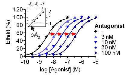
To record a shield plot and to calculate the p A ₂ value from it, the antagonist is incubated in separate experiments in different concentrations in a pharmacological test system (e.g. cell culture or tissue ) or, in animal experiments , administered to a test animal . Then, by adding or administering increasing concentrations of an agonist, the agonist concentration is usually determined at which a half-maximum effect can be observed ( EC ₅₀ value). This value depends on the concentration of the antagonist and increases as the antagonist concentration increases. The ratio of EC ₅₀ value in presence of antagonist, and EC ₅₀ value in absence of antagonist is expressed as the concentration ratio ( concentration ratio ) r denotes:

${\displaystyle r={\frac {EC_{50}(+Antagonist)}{EC_{50}(-Antagonist)}}}$

The concentration ratio determined for different antagonist concentrations is plotted in a diagram as log ( r -1) against the logarithm of the molar antagonist concentration . The point of intersection of the compensation function with the abscissa corresponds to the p A ₂ value of the antagonist if there is a linearity and a slope of the regression line of approximately m = 1 .

Alternatively, a shield plot based on any EC _X value is theoretically possible.

Determination of the p A ₂ value with the aid of the Schild plot: increasing antagonist concentrations lead to a right shift of the concentration-effect curve and to a decrease in the p EC ₅₀ value of the agonist. From this shift to the right, the concentration ratio r can be calculated, which is entered as log ( r -1) against the logarithm of the molar antagonist concentration in the Schild plot (embedded figure) and is used to determine the p A ₂ value.

Interpretations

In addition to determining the p A ₂ value, the Schild plot also enables statements to be made about the qualitative type of antagonism. A linearity of the compensation function and a slope of the best-fit straight line of m = 1 is a good indication of the existence of a competitive antagonism . Under these conditions the determined p A ₂ value corresponds to the affinity constant p K _{B of} the antagonist.

Deviation from linearity

If the compensation function does not show a linear course, then, even if all other prerequisites are met (in particular a parallel right shift of the agonist's concentration-activity curve caused by the antagonist), one can no longer speak of a purely competitive antagonism. If the compensation function has two or more linear sections, this indicates a competition between agonist and antagonist for two or more binding sites on the receptor.

Deviation from the slope m = 1

If, with at least approximate linearity, the compensation function has a slope of m > 1, which in practice means a disproportionate decrease in the effect of the antagonist with decreasing concentration, this indicates an inactivation or an uptake of the antagonist under experimental conditions. This phenomenon occurs even if the incubation time of the antagonist is insufficient.

The more common case that the regression line in the Schild plot has a gradient of m  <1 can be attributed, among other things, to an inactivation or an uptake of the agonist used. Competition between antagonist and agonist for different binding sites with different binding affinities for these ligands can also lead to a straight line with a slope of m  <1.

Alternatives

Alternative methods are e.g. B. the Gaddum equation according to John Gaddum and the Cheng-Prusoff equation .

literature

• O. Arunlakshana, HO Schild: Some quantitative uses of drug antagonism . In: Br. J. Pharmacol. , 1959, 14, pp. 48-58.
• T. Kenakin: Pharmacological analysis of drug-receptor interaction . 2nd ed. Raven Press, New York 1993.

Individual evidence

1. ^ RR Neubig, M. Spedding, T. Kenakin, A. Christopoulos: International Union of Pharmacology Committee on Receptor Nomenclature and Drug Classification. International Union of Pharmacology Committee on Receptor Nomenclature and Drug Classification. XXXVIII. Update on terms and symbols in quantitative pharmacology. In: Pharmacol Rev. , 2003, Vol. 55, No. 4, pp. 597-606. PMID 14657418 . PDF .
2. ↑ S. Lazareno, NJ Birdsall: Estimation of competitive antagonist affinity from functional inhibition curves using the Gaddum, Schild and Cheng-Prusoff equations. In: Br J Pharmacol. , 1993, Vol. 109, No. 4, pp. 1110-1119. PMID 8401922 ; PMC 2175764 (free full text).
3. ↑ TF Webster: Mixtures of endocrine disruptors: How similar must mechanisms be for concentration addition to apply? In: Toxicology , 2013. PMID 23357612 , doi: 10.1016 / j.tox.2013.01.009 .
4. ↑ TL Williams, DA Smith NR Burton, TW Stone: amino acid pharmacology in neocortical slices: evidence for bimolecular actions from on extension of the Hill and Gaddum Shield equations. In: Br J Pharmacol. , 1988, Vol. 95, No. 3, pp. 805-810. PMID 2905185 ; PMC 1854217 (free full text).