Goldfeld-Quandt test

The Goldfeld-Quandt test is a statistical test for heteroscedasticity (non-constant variance of the confounding variables ) in regression analysis . The test is based on the comparison of two sample halves. It was named after Stephen Goldfeld and Richard E. Quandt.

Action

Procedure for the Goldfeld-Quandt test

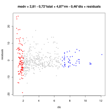
The sample is divided into two subsets for an explanatory variable, see graphic. The two subsets must be disjoint so that no observations occur in both subsets. However, the two subsets together do not have to encompass the entire sample. In the graphic is e.g. B. the middle part of the observations in no subset (gray). A regression is estimated for both subsets and the variance of the residuals is calculated. Then the sample variance of the residuals for i = 1.2 is determined (with ) for each subset and the test value is compared with a critical value from the F-distribution . The example shows heteroscedasticity because the regression for one subset shows a high residual variance (red), while the regression for the other subset shows a low residual variance (blue). ${\displaystyle {s_{i}^{2}}}$ ${\displaystyle s_{1}^{2}>s_{2}^{2}}$ ${\displaystyle {\tfrac {s_{1}^{2}}{s_{2}^{2}}}}$

Mathematical formulation

requirement

In the classic regression model, or with and applies . The test is sensitive to violations of the normal distribution of the residuals. ${\displaystyle Y_{i1}=f_{1}(x_{i1})+U_{i1}}$ ${\displaystyle Y_{i2}=f_{2}(x_{i2})+U_{i2}}$ ${\displaystyle U_{i1}\sim {\mathcal {N}}(0,\sigma _{1}^{2})}$ ${\displaystyle U_{i2}\sim {\mathcal {N}}(0,\sigma _{2}^{2})}$

Hypotheses and test statistics

The null and alternative hypotheses are

${\displaystyle H_{0}:\sigma _{1}^{2}=\sigma _{2}^{2}=\sigma ^{2},}$(Presence of homoscedasticity) vs. (Presence of heteroscedasticity). ${\displaystyle H_{1}:\sigma _{1}^{2}\neq \sigma _{2}^{2}}$

The distribution of the test statistic results as

${\displaystyle F={\frac {S_{1}^{2}}{S_{2}^{2}}}\sim F_{n_{1}-k;n_{2}-k}}$

with the number of observations in the th part and the number of estimated regression parameters as well ${\displaystyle n_{i}}$ ${\displaystyle i}$ ${\displaystyle k}$

${\displaystyle S_{i}^{2}={\frac {1}{n_{i}-k}}\sum _{j=1}^{n_{i}}U_{ji}^{2}}$.

The null hypothesis (homoscedasticity) is rejected if the test value is greater than the critical value from the F-distribution with and degrees of freedom and a predefined level of significance . ${\displaystyle F_{n_{1}-k;n_{2}-k}(1-\alpha )}$ ${\displaystyle n_{1}-k}$ ${\displaystyle n_{2}-k}$ ${\displaystyle \alpha }$

example

variable	meaning
medv	Median purchase price of a house in US $ 1000
lstat	Proportion of the lower class population
rm	Average number of rooms
dis	Weighted distance to the five most important employment centers

For the example, linear regressions were performed on the Boston Housing data set . The variables on the right were collected for each of the 506 districts and a multiple linear regression was carried out:

${\displaystyle medv_{i}=2,8083-0{,}7233lstat_{i}+4{,}8734rm_{i}-0{,}4613dis_{i}+{\hat {u}}_{i}}$.

If you plot the residuals against the variable dis (graphic above) you can see that the variance of the residuals decreases when the values ​​of dis increase. The data is now divided into two parts: the red and the blue part. Then you fit two regression models and calculate the sum of the squared residuals.

red	${\displaystyle medv_{i1}=+56{,}116-1{,}002lstat_{i1}+0{,}664rm_{i1}-14{,}106dis_{i1}+{\hat {u}}_{i1}}$
	${\displaystyle s_{1}^{2}={\frac {1}{n_{1}-k}}\sum _{i=1}^{n_{1}}{\hat {u}}_{i1}^{2}={\frac {4899{,}807}{112-4}}=45{,}369}$
blue	${\displaystyle medv_{i2}=-40{,}858-0{,}044lstat_{i2}+9{,}895rm_{i2}+0{,}233dis_{i2}+{\hat {u}}_{i2}}$
	${\displaystyle s_{2}^{2}={\frac {1}{n_{2}-k}}\sum _{i=1}^{n_{2}}{\hat {u}}_{i2}^{2}={\frac {179{,}927}{49-4}}=3{,}998}$

Then the test value results from and the critical value for a significance level results from the F-distribution with 108 and 45 degrees of freedom . Since the test value is greater than the critical value, the null hypothesis of homoscedasticity must be rejected. ${\displaystyle f={\tfrac {45{,}369}{3,998}}=11{,}347}$ ${\displaystyle \alpha =5\,\%}$ ${\displaystyle c=1{,}548}$

literature

• William E. Griffiths, R. Carter Hill, George G. Judge: Learning and Practicing Econometrics . 1st edition. 1993, ISBN 0-471-51364-4 , p. 494 ff.

Individual evidence

1. ↑ Stephen M. Goldfeld, RE Quandt: Some Tests for Homoscedasticity . In: Journal of the American Statistical Association . 60, No. 310, June 1965, pp. 539-547. JSTOR 2282689 . doi : 10.1080 / 01621459.1965.10480811 .