Demand function

Fig. 1) Example of a (linear) demand curve

In economics , the demand function is a mathematical function which, for a given price of a good, indicates the amount that is in demand at that price. It is usually shown graphically with interchanged coordinate axes : the price is shown on the vertical axis and the quantity is shown on the horizontal axis. A distinction is made between individual and aggregated demand functions. The former record the demand behavior of a person, the latter record the demand behavior of all market participants.

The demand function is often used in conjunction with the supply function to determine the market equilibrium - that is, the price-quantity combination in which the demand for the good corresponds to the quantity offered at this price.

general definition

A demand function is generally a function , . It is usually assumed to be a linear function ${\ displaystyle D \ colon \ mathbb {R} _ {+} \ to \ mathbb {R} _ {+}}$ ${\ displaystyle p \ mapsto D (p)}$

{\ displaystyle D (p) = \ operatorname {max} \ left \ {a-bp, 0 \ right \}}

The parameters a and b represent the axis intercept and the slope . The maximum function expresses that the function is generally represented by; but when the demand becomes negative it takes the value zero, since usually no negative demand exists. It is usually assumed to be strictly monotonically decreasing , that is, as the price increases, the demand should also decrease. A special case that is usually negligible is represented by so-called Giffen goods , the demand for which is increasing in price. ${\ displaystyle a-bp}$

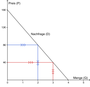
The price that corresponds to a demand of zero is called the prohibitive price ; In the graphic example in Fig. 1, this is € 16.

The maximum amount that is demanded - assuming a falling course of the demand curve, this is nothing other than the amount that is demanded when the price is zero - is called the saturation amount ; it amounts to four units of the property in Fig. 1.

Horizontal and vertical interpretation of the individual demand function

The fact that the demand function is usually represented with swapped coordinate axes means that the resulting curve can only be read from the price axis (see below: horizontal interpretation ); Finally, a different graphical representation does not change the fact that the price is functionally mapped to the quantity (and not the quantity to the price). However, the individual demand curve can actually also be interpreted vertically .

Note, however, that this is generally not the case for aggregate demand (see section below) .

Fig. 2) Horizontal interpretation of the demand function ("demand as a function of price")

Fig. 3) Vertical interpretation of the demand function ("price as a function of demand")

Horizontal interpretation

The horizontal interpretation of the demand function is the one that most closely follows the current understanding. It strictly follows the functional form of the demand function: Based on the price, the question of how high the resulting demand is. For example, Fig. 2 shows that consumers are willing to purchase 2 units at a price of € 8; at a price of € 4 they would be willing to buy 3 units.

Vertical interpretation

With a vertical interpretation, the example can be read as follows (Fig. 3): In order for the demand to be 3 units, the price must be € 4. Or to put it another way: The price that consumers are willing to pay for the third unit is € 4.

consequence

1 follows from the co-existence of horizontal and vertical interpretation that one figure. So can also be interpreted as if it were a non-function , whose axes are reversed, but simply a function , in ordinary representation. This function is known as the price-sales function . It is the inverse function of the demand function. Be for example ${\ displaystyle D \ colon \ mathbb {R} _ {+} \ to \ mathbb {R} _ {+}}$ ${\ displaystyle p \ mapsto D (p)}$ ${\ displaystyle p \ colon \ mathbb {R} _ {+} \ to \ mathbb {R} _ {+}}$ ${\ displaystyle Q \ mapsto p (Q)}$ ${\ displaystyle p (Q)}$

{\ displaystyle D (p) = Q = 4-0 {,} 25p}

,

then the inverse function is

{\ displaystyle p (Q) = 16-4Q}

.

This is precisely the function that corresponds to the “swapped” demand function from the example in Fig. 1 (but also allows a horizontal interpretation).

Aggregated demand curve

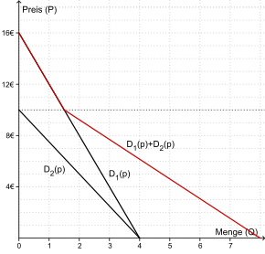
Fig. 4) Addition of demand functions. The market demand curve resulting from the individual curves is shown in red.

While individual demand curves indicate the demand for a good by an individual / household, aggregated demand curves represent the demand by all market participants; one speaks accordingly of market demand. The aggregation is done graphically by adding the individual requests. It should be noted, however, that in Fig. 4, for example, you cannot add vertically (the prices cannot be added), but only horizontally. Since there are no negative inquiries, the demand from person 2 can only be added below a price of 10 €; One of the consequences of this is that the aggregation usually results in a “kink” in the function.

In principle, demand can also be aggregated vertically (via price). This is e.g. B. the case in determining a social demand for public goods . Due to the non-rivalry of these goods, it makes sense to consider the marginal willingness of all buyers to pay. If the individually rational demands are zero, but the social demand is greater, this can be a reason for the state to intervene in the market and regulate the provision of the goods (e.g. via taxes).

Marshallian and Hicksian demand

In the household theory of microeconomics, the aggregated demand function results from the individual benefit maximization of the households. The individual demand for a good depends on two factors: on the one hand, on the prices of all goods, on the other hand, on the budget available to the household.

Web links

The demand . In: <mikro> online, accessed on February 10, 2012.

literature

Friedrich Breyer: Microeconomics. An introduction. 5th edition. Springer, Heidelberg a. a. 2011, ISBN 978-3-642-22150-7 .
Jürgen Eichberg: Basics of microeconomics. Mohr Siebeck, 2004, ISBN 978-3-16-148167-3 .
Hal Varian : Intermediate Microeconomics. A modern approach. 8th edition. WW Norton, New York and London 2010, ISBN 978-0-393-93424-3 .

Individual evidence

↑ Their existence requires that the demand function over the area of interest is bijective .

[1] Their existence requires that the demand function over the area of interest is bijective .