BDF process

The BDF method ( English B ackward D ifferentiation F ormulas ) are linear multi-step process for the numerical solution of initial value problems of ordinary differential equations :

${\displaystyle y'(x)=f(x,y(x)),\quad y(x_{0})=y_{0},\quad y\colon \mathbb {R} \to \mathbb {R} ^{n}}$.

The following is calculated for an approximate solution at the intermediate points : ${\displaystyle y(x)}$ ${\displaystyle x_{i}}$

${\displaystyle y_{i}\approx y(x_{i})\quad i=1,\dotsc ,m}$.

The methods were introduced in 1952 by Charles Francis Curtiss and Joseph Oakland Hirschfelder and have been widely used as solvers for stiff initial value problems since the publication of C. William Gear in 1971 .

description

In contrast to the Adams-Moulton method , in the BDF method the right side is not approximated by an interpolation polynomial , instead a polynomial with (maximum) degree is constructed , which interpolates the last approximations to the solution as well as the unknown value : ${\displaystyle q_{k}}$ ${\displaystyle k}$ ${\displaystyle k}$ ${\displaystyle y_{n},\dotsc ,y_{n+k-1}}$ ${\displaystyle y_{n+k}}$

${\displaystyle q_{k}(x_{i})=y_{i},\quad {\text{für }}i=n,\dots ,n+k}$.

In addition, one demands that the interpolation polynomial solves the given differential equation at the point , i.e. that it holds ${\displaystyle q_{k}}$ ${\displaystyle x_{n+k}}$

${\displaystyle q_{k}'(x_{n+k})=f(x_{n+k},y_{n+k})}$,

and thus receives a non-linear system of equations for determining the implicitly given value . ${\displaystyle y_{n+k}}$

Lagrange representation

One possibility for the representation of the interpolation polynomial is the Lagrange representation . The Lagrange base polynomials with the support points are defined by ${\displaystyle q_{k}}$ ${\displaystyle k+1}$ ${\displaystyle x_{n},\dots ,x_{n+k}}$

${\displaystyle l_{j}(x_{n+i})=\delta _{ji}={\begin{cases}1&{\text{falls }}j=i,\\0&{\text{falls }}j\neq i.\end{cases}}}$

where is the Kronecker delta . Because of this, the representation follows directly ${\displaystyle \delta _{ji}}$ ${\displaystyle q_{k}(x_{n+i})=\sum _{j=0}^{k}l_{j}(x_{n+j})y_{n+j}=y_{n+i}}$

${\displaystyle q_{k}(x)=\sum _{j=0}^{k}l_{j}(x)y_{n+j}}$.

The requirement now gives the linear recursion formula for the BDF method: ${\displaystyle q_{k}'(x_{n+k})=f(x_{n+k},y_{n+k})}$

${\displaystyle \sum _{j=0}^{k}\alpha _{j}y_{n+j}=f(x_{n+k},y_{n+k})}$,

where the coefficients are given by ${\displaystyle \alpha _{j}}$

${\displaystyle \alpha _{j}=l_{j}'(x_{n+k}),\quad j=0,\dots ,k}$.

Alternative Lagrange representation

Alternatively, consider the Lagrange base polynomials defined by

${\displaystyle L_{j}(-s)=\delta _{js}={\begin{cases}1&{\text{falls }}j=s,\\0&{\text{falls }}j\neq s.\end{cases}}}$

The illustration follows

${\displaystyle q_{k}(x_{n+k}+sh)=\sum _{j=0}^{k}L_{k-j}(s)y_{n+j}}$.

This is the distance between the support points and the constant step size of the method. With the requirement of being here ${\displaystyle h=x_{i+1}-x_{i}}$ ${\displaystyle q_{k}'(x_{n+k})=f(x_{n+k},y_{n+k})}$

${\displaystyle q_{k}'(x)={\frac {d}{dx}}q_{k}(x)={\frac {d}{d(sh)}}q_{k}(x_{n+k}+sh)={\frac {1}{h}}{\frac {d}{ds}}q_{k}(x_{n+k}+sh)}$

applies, one now obtains for the calculation of the coefficients ${\displaystyle \alpha _{j}}$

${\displaystyle \alpha _{j}=L_{k-j}'(0),\quad j=0,\dots ,k}$

and with it the recursion formula

${\displaystyle \sum _{j=0}^{k}L_{k-j}'(0)y_{n+j}=hf(x_{n+k},y_{n+k})}$

Newton representation

The Newtonian representation of the interpolation polynomial uses backward differences, which are recursively defined by ${\displaystyle q_{k}}$

${\displaystyle \nabla ^{0}y_{i}=y_{i},\quad \nabla ^{j+1}y_{i}=\nabla ^{j}y_{i}-\nabla ^{j}y_{i-1}.}$

This can be written as ${\displaystyle q_{k}}$

${\displaystyle q_{k}\left(x_{n+k}+sh\right)=\sum _{j=0}^{k}(-1)^{j}{\binom {-s}{j}}\nabla ^{j}y_{n+k}}$.

This formula leads because of for on the representation ${\displaystyle \left.{\frac {d}{ds}}(-1)^{j}{\binom {-s}{j}}\right|_{s=0}={\frac {1}{j}}}$ ${\displaystyle j=1,\dots ,k}$

${\displaystyle \sum \limits _{j=1}^{k}{\frac {1}{j}}\nabla ^{j}y_{n+k}=hf(x_{n+k},y_{n+k})}$

the BDF process.

Calculation formulas

All the representations of the calculation formulas considered above are equivalent, since they only used different types of representation of the unique interpolation polynomial . For the implicit calculation formulas of the BDF (k) method are: ${\displaystyle q_{k}}$ ${\displaystyle k\leq 6}$

• BDF (1) - implicit Euler method:

${\displaystyle y_{n+1}-y_{n}=hf(x_{n+1},y_{n+1})}$

• BDF (2):

${\displaystyle 3y_{n+2}-4y_{n+1}+y_{n}=2hf(x_{n+2},y_{n+2})}$

• BDF (3):

${\displaystyle 11y_{n+3}-18y_{n+2}+9y_{n+1}-2y_{n}=6hf(x_{n+3},y_{n+3})}$

• BDF (4):

${\displaystyle 25y_{n+4}-48y_{n+3}+36y_{n+2}-16y_{n+1}+3y_{n}=12hf(x_{n+4},y_{n+4})}$

• BDF (5):

${\displaystyle 137y_{n+5}-300y_{n+4}+300y_{n+3}-200y_{n+2}+75y_{n+1}-12y_{n}=60hf(x_{n+5},y_{n+5})}$

• BDF (6):

${\displaystyle 147y_{n+6}-360y_{n+5}+450y_{n+4}-400y_{n+3}+225y_{n+2}-72y_{n+1}+10y_{n}=60hf(x_{n+6},y_{n+6})}$

properties

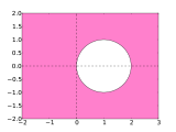
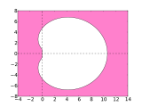
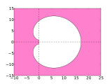
The BDF methods are all implicit because the unknown value goes into the equation. BDF (k) has exactly the consistency order k . The BDF (1) method is the implicit Euler method . This and BDF (2) are A-stable , the higher-order methods are A ( ) -stable, with the opening angle decreasing with the higher order. In particular, BDF (2) is very popular for the calculation of stiff differential equations due to its optimal properties with regard to the second Dahlquist barrier . For k <6 , the methods are stable and consistent and therefore also convergent. The greatest incentive of the BDF methods is their large stability areas, which is why they are suitable for use in solving rigid initial value problems. For k> 6 the methods are unstable. ${\displaystyle y_{n+k}}$ ${\displaystyle \alpha }$ ${\displaystyle \alpha }$

• Stability areas of the BDF process
• 

  BDF1

• 

  BDF2

• 

  BDF3

• 

  BDF4

• 

  BDF5

• 

  BDF6

literature

• E. Hairer, Syvert P. Nørsett, Gerhard Wanner: Solving Ordinary Differential Equations I, Nonstiff Problems , Springer Verlag, ISBN 3540566708
• E. Hairer, G. Wanner: Solving Ordinary Differential Equations II, Stiff problems , Springer Verlag, ISBN 3-540-60452-9
• HR Schwarz, N. Köckler: Numerical Mathematics , Teubner (2004)
• Curtiss, Hirschfelder Integration of stiff equations , Proc. Nat. Acad. Sci. USA, Vol. 38, 1952, 235-243.

Web links

• Gear, Backward Differentiation Formulas, Scholarpedia