Polynomial interpolation

7th degree interpolation polynomial

In numerical mathematics , polynomial interpolation is the search for a polynomial which runs exactly through specified points (e.g. from a series of measurements). This polynomial is called the interpolation polynomial and is said to interpolate the given points.

Applications

Polynomials can be integrated and derived very easily. That is why interpolating polynomials appear in many places in numerical mathematics, for example in numerical integration and correspondingly in methods for the numerical solution of ordinary differential equations .

Problem

For given pairs of values with different interpolation points in pairs , a polynomial of the maximum -th degree is sought that contains all equations ${\displaystyle n+1}$ ${\displaystyle (x_{i},\,f_{i})}$ ${\displaystyle x_{i}}$ ${\displaystyle P}$ ${\displaystyle n}$

${\displaystyle P(x_{i})=f_{i},\quad i=0,\dotsc ,n}$

Fulfills. Such a polynomial always exists and is uniquely determined, as shown below.

In the case of the interpolation problem, the polynomials with degrees or less must be looked for in the vector space , in short . Is a base of , the equations yield a linear equation system for the coefficients of the basis representation . Since one and the same polynomial can be represented differently, depending on which base is chosen for the vector space , one can get very different systems of equations. If you choose for the standard basis , i.e. for the representation , you get a system of equations with the Vandermonde matrix : ${\displaystyle P}$ ${\displaystyle \Pi _{n}}$ ${\displaystyle n}$ ${\displaystyle P\in \Pi _{n}}$ ${\displaystyle \phi _{0},\dotsc ,\phi _{n}}$ ${\displaystyle \Pi _{n}}$ ${\displaystyle P(x_{i})=f_{i}}$ ${\displaystyle P=\sum _{k=0}^{n}a_{k}\phi _{k}}$ ${\displaystyle \Pi _{n}}$ ${\displaystyle \Pi _{n}}$ ${\displaystyle \left\{x^{k}\mid 0\leq k\leq n\right\}}$ ${\displaystyle P}$ ${\displaystyle P(x)=\sum _{k=0}^{n}a_{k}x^{k}}$

${\displaystyle {\begin{pmatrix}1&x_{0}&\cdots &x_{0}^{n}\\\vdots &\vdots &\ddots &\vdots \\1&x_{n}&\cdots &x_{n}^{n}\end{pmatrix}}{\begin{pmatrix}a_{0}\\\vdots \\a_{n}\end{pmatrix}}={\begin{pmatrix}f_{0}\\\vdots \\f_{n}\end{pmatrix}}}$.

This is regular if the support points are different in pairs, the system of equations can then be solved clearly. Thus the existence and uniqueness of the polynomial sought is always guaranteed. Despite the theoretically simple representation, this system of equations is not used in practice for calculating the interpolation polynomial, since its solution is complex and it is also generally poorly conditioned . ${\displaystyle x_{i}}$ ${\displaystyle P\in \Pi _{n}}$

Solution method

The above system of equations could be solved, for example, with the Gaussian elimination method. With (see Landau symbols ) the effort would be comparatively large. If a different basis than the standard basis for describing the polynomial is selected , the effort can be reduced. ${\displaystyle {\mathcal {O}}\left(n^{3}\right)}$ ${\displaystyle P}$

Lagrangian interpolation formula

Exemplary Lagrangian basis functions for x ₀ = 0, x ₁ = 1, x ₂ = 2, x ₃ = 3 (n = 3)

A representation in the Lagrange basis is more favorable for theoretical considerations . The basic functions are the Lagrange polynomials

${\displaystyle \ell _{i}(x)=\prod _{\begin{smallmatrix}j=0\\j\neq i\end{smallmatrix}}^{n}{\frac {x-x_{j}}{x_{i}-x_{j}}}={\frac {x-x_{0}}{x_{i}-x_{0}}}\cdots {\frac {x-x_{i-1}}{x_{i}-x_{i-1}}}\cdot {\frac {x-x_{i+1}}{x_{i}-x_{i+1}}}\cdots {\frac {x-x_{n}}{x_{i}-x_{n}}}\,,}$

which are defined so that

${\displaystyle \ell _{i}(x_{k})=\delta _{ik}=\left\{{\begin{matrix}1&{\text{falls }}i=k\\0&{\text{falls }}i\neq k\end{matrix}}\right.}$

applies, where the Kronecker delta represents. The matrix thus corresponds exactly to the identity matrix . The solution to the interpolation problem can then simply be given as ${\displaystyle \delta _{ik}}$ ${\displaystyle \left(\ell _{i}\left(x_{j}\right)\right)_{i,j=0,1,\dotsc ,n}}$

${\displaystyle P(x)=\sum _{i=0}^{n}f_{i}\ell _{i}\left(x\right)}$

with the support values . This is often used to prove the existence of the solution to the interpolation problem. One advantage of the Lagrange basis is that the basis functions are independent of the support values . As a result, different sets of interpolation values with the same interpolation points can be interpolated quickly once the basic functions have been determined. A disadvantage of this representation, however, is that all base vectors have to be completely recalculated when a single support point is added, which is why this method is too expensive for most practical purposes. In digital signal processing, Lagrange interpolation is used under the name "Farrow Filter" for adaptive resampling. ${\displaystyle f_{i}}$ ${\displaystyle \ell _{i}}$ ${\displaystyle f_{i}}$ ${\displaystyle f_{i}}$ ${\displaystyle x_{i}}$ ${\displaystyle \ell _{i}}$

Barycentric interpolation formula

The Lagrangian interpolation formula can be transformed into the practically more relevant barycentric interpolation formula

${\displaystyle P(x)={\frac {\sum _{j=0}^{n}{\frac {\lambda _{j}f_{j}}{x-x_{j}}}}{\sum _{j=0}^{n}{\frac {\lambda _{j}}{x-x_{j}}}}}\,,}$

where the barycentric weights are defined as follows

${\displaystyle \lambda _{j}:=\prod _{\begin{smallmatrix}i=0\\i\neq j\end{smallmatrix}}^{n}{\frac {1}{x_{j}-x_{i}}}\,.}$

The weights can be precalculated for given support points so that the effort for the evaluation of is only at . When adding a new support point, the weights must be redetermined. This has an expense compared to redetermining the Lagrangian polynomials of . ${\displaystyle \left(x_{i}\right)_{i}}$ ${\displaystyle \left(\lambda _{i}\right)_{i}}$ ${\displaystyle P(x)}$ ${\displaystyle {\mathcal {O}}(n)}$ ${\displaystyle {\mathcal {O}}(n)}$ ${\displaystyle {\mathcal {O}}\left(n^{2}\right)}$

Newton's algorithm

In this procedure, the polynomial is represented in Newton-based so that the coefficients can be determined efficiently using the divided differences scheme . An efficient evaluation of the polynomial can then take place with the help of the Horner scheme . ${\displaystyle P}$

Approach: Newton basis

As an approach for the interpolation polynomial you are looking for , you choose the Newton basis functions and with , so that it is represented with the Newton interpolation formula ${\displaystyle P}$ ${\displaystyle N_{0}(x)=1}$ ${\displaystyle \textstyle N_{i}(x)=\prod _{j=0}^{i-1}\left(x-x_{j}\right)=\left(x-x_{0}\right)\dotsm \left(x-x_{i-1}\right)}$ ${\displaystyle i=1,\dotsc ,n}$ ${\displaystyle P}$

${\displaystyle P(x)=\sum _{i=0}^{n}c_{i}\cdot N_{i}(x)=c_{0}+c_{1}\left(x-x_{0}\right)+c_{2}\left(x-x_{0}\right)\left(x-x_{1}\right)+\dotsb +c_{n}\left(x-x_{0}\right)\dotsm \left(x-x_{n-1}\right)}$

The system of equations then has the form ${\displaystyle P(x_{i})=f_{i}}$

${\displaystyle {\begin{pmatrix}1&&&&0\\1&(x_{1}-x_{0})&&&\\1&(x_{2}-x_{0})&(x_{2}-x_{0})(x_{2}-x_{1})&&\\\vdots &\vdots &&\ddots &\\1&(x_{n}-x_{0})&\cdots &&\prod _{i=0}^{n-1}(x_{n}-x_{i})\\\end{pmatrix}}\cdot {\begin{pmatrix}c_{0}\\\vdots \\c_{n}\end{pmatrix}}={\begin{pmatrix}f_{0}\\\vdots \\f_{n}\end{pmatrix}}}$

In contrast to the Vandermonde matrix when the standard basis is selected, when the Newton basis is selected, a simply structured lower triangular matrix is ​​obtained and the system of equations can be solved easily. ${\displaystyle \left\{x^{k}\mid 0\leq k\leq n\right\}}$

Determination of the coefficients: scheme of the divided differences

The coefficients are not determined directly from the above system of equations, but more efficiently using the divided differences. By induction one proves with the recursion formula of Aitken that holds for the coefficients ${\displaystyle c_{i}}$ ${\displaystyle c_{i}}$

${\displaystyle c_{i}=\left[x_{0},\dotsc ,x_{i}\right]f}$.

Here, for the divided differences defined recursively ${\displaystyle i<j}$ ${\displaystyle \left[x_{i},\dotsc ,x_{j}\right]f}$

${\displaystyle \left[x_{i}\right]f=f_{i}\qquad }$

${\displaystyle \left[x_{i},\dotsc ,x_{j}\right]f={\frac {\left[x_{i+1},\dotsc ,x_{j}\right]f-\left[x_{i},\dotsc ,x_{j-1}\right]f}{x_{j}-x_{i}}}}$.

The notation with an appended is explained by the fact that an unknown function is often assumed that is to be interpolated with known function values. ${\displaystyle f}$ ${\displaystyle f}$ ${\displaystyle f_{i}=f\left(x_{i}\right)}$

The recursive calculation of the divided differences can be illustrated as follows. The coefficients you are looking for are exactly the top diagonal line: ${\displaystyle c_{i}}$

${\displaystyle {\begin{array}{crcrccrcrc}[x_{0}]f\\&\searrow \\{}[x_{1}]f&\rightarrow &[x_{0},x_{1}]f\\&\searrow &&\searrow \\{}[x_{2}]f&\rightarrow &[x_{1},x_{2}]f&\rightarrow &[x_{0},x_{1},x_{2}]f\\{}\vdots &\vdots &\vdots &\vdots &\vdots &\ddots \\{}&\searrow &&\searrow &&&\searrow \\{}[x_{n-1}]f&\rightarrow &[x_{n-2},x_{n-1}]f&\rightarrow &[x_{n-3},x_{n-2},x_{n-1}]f&\cdots &\rightarrow &[x_{0},\ldots ,x_{n-1}]f\\&\searrow &&\searrow &&&\searrow &&\searrow \\{}[x_{n}]f&\rightarrow &[x_{n-1},x_{n}]f&\rightarrow &[x_{n-2},x_{n-1},x_{n}]f&\cdots &\rightarrow &[x_{1},\ldots ,x_{n}]f&\rightarrow &[x_{0},\ldots ,x_{n}]f\end{array}}}$

Obviously, when adding a further point to the value pairs in the above scheme, only one more line needs to be added to calculate the additional coefficient . The previously determined coefficients do not have to be recalculated. ${\displaystyle n+1}$ ${\displaystyle \left(x_{i},f_{i}\right)}$ ${\displaystyle \left(x_{n+1},f_{n+1}\right)}$ ${\displaystyle c_{n+1}=\left[x_{0},\dotsc ,x_{n+1}\right]f}$ ${\displaystyle c_{0},\dotsc ,c_{n}}$

As an alternative to the recursive definition above, in one of Marsden's articles, for example, the divided difference of a sufficiently often differentiable function is defined as the unambiguous coefficient to the highest power of a polynomial -th degree that interpolates at the points . If a value occurs in the sequence with the multiplicity , the derivatives of the polynomial should interpolate the derivatives of the function at this point up to the order . It is therefore true ${\displaystyle \left[x_{0},\dotsc ,x_{n}\right]f}$ ${\displaystyle f}$ ${\displaystyle x}$ ${\displaystyle n}$ ${\displaystyle p(x)}$ ${\displaystyle f}$ ${\displaystyle x_{0},\dotsc ,x_{n}}$ ${\displaystyle x_{0},\dotsc ,x_{n}}$ ${\displaystyle \nu \geq 1}$ ${\displaystyle f}$ ${\displaystyle \nu -1}$

${\displaystyle \left[x_{0},\dotsc ,x_{k}\right]f={\frac {f^{(k)}(x^{*})}{k!}}\qquad {\text{falls}}\quad x^{*}:=x_{0}=\dotsb =x_{k}\,.}$

Evaluation of the polynomial: Horner scheme

Once the coefficients of the interpolation polynomial are known, it can be evaluated efficiently using Horner's scheme . To do this, one writes in the form (simple transformation of Newton's interpolation formula) ${\displaystyle c_{i}}$ ${\displaystyle P}$ ${\displaystyle P}$

${\displaystyle P(x)=\left(\dotso \left(c_{n}\left(x-x_{n-1}\right)+c_{n-1}\right)\left(x-x_{n-2}\right)+\dotsb +c_{1}\right)\left(x-x_{0}\right)+c_{0}}$,

so that can be computed recursively through ${\displaystyle P(x)}$

${\displaystyle {\begin{aligned}b_{n}&=c_{n}\\b_{i}&=b_{i+1}\left(x-x_{i}\right)+c_{i},\qquad i=n-1,\dotsc ,0\\P(x)&=b_{0}\end{aligned}}}$

This requires an effort of . ${\displaystyle {\mathcal {O}}(n)}$

Neville-Aitken's algorithm

Similar to Newton's algorithm , the Neville-Aitken algorithm calculates the solution recursively. For this purpose, denote the uniquely determined interpolation polynomial -th degree for the support points , where is. Aitken's recursion formula then applies: ${\displaystyle p\left(f|x_{i},\dotsc ,x_{j}\right)}$ ${\displaystyle k}$ ${\displaystyle k+1}$ ${\displaystyle \left(x_{i},f_{i}\right),\dotsc ,\left(x_{j},f_{j}\right)}$ ${\displaystyle k=j-i}$

${\displaystyle {\begin{aligned}p(f|x_{i})(x)&\equiv f_{i},\\p\left(f|x_{i},\dotsc ,x_{j}\right)(x)&\equiv {\frac {\left(x-x_{i}\right)p\left(f|x_{i+1},\dotsc ,x_{j}\right)(x)-\left(x-x_{j}\right)p\left(f|x_{i},\dotsc ,x_{j-1}\right)(x)}{x_{j}-x_{i}}}.\end{aligned}}}$

It can be proven by substituting , which verifies that the right hand side of the equation satisfies the interpolation condition. The uniqueness of the interpolation polynomial then provides the assertion. ${\displaystyle x_{i}}$

With Neville's scheme, the evaluation of can then be done recursively: ${\displaystyle p\left(f|x_{0},\dotsc ,x_{n}\right)(x)=P(x)}$

${\displaystyle {\begin{array}{crcrccrcrc}p(f|x_{0})\\&\searrow \\p(f|x_{1})&\rightarrow &p(f|x_{0},x_{1})\\&\searrow &&\searrow \\p(f|x_{2})&\rightarrow &p(f|x_{1},x_{2})&\rightarrow &p(f|x_{0},x_{1},x_{2})\\\vdots &&\vdots &&\vdots &\ddots \\&\searrow &&\searrow &&&\searrow \\p(f|x_{n-1})&\rightarrow &p(f|x_{n-2},x_{n-1})&\rightarrow &p(f|x_{n-3},x_{n-2},x_{n-1})&\cdots &\rightarrow &p(f|x_{0},\dotsc ,x_{n-1})\\&\searrow &&\searrow &&&\searrow &&\searrow \\p(f|x_{n})&\rightarrow &p(f|x_{n-1},x_{n})&\rightarrow &p(f|x_{n-2},x_{n-1},x_{n})&\cdots &\rightarrow &p(f|x_{1},\dotsc ,x_{n})&\rightarrow &p(f|x_{0},\dotsc ,x_{n})\end{array}}}$

Comparison of the solution methods

If you want to determine all the coefficients of the interpolation polynomial , Newton's algorithm offers the least effort required for this . The polynomial determined in this way can then be evaluated with operations at one point. This is why Newton's algorithm is well suited when the interpolation polynomial is to be evaluated in many places. Additional support points can also be added efficiently. If the interpolation points or the interpolation values ​​are too close to one another, however, there is a risk of being erased when determining the divided differences. ${\displaystyle P}$ ${\displaystyle {\mathcal {O}}\left(n^{2}\right)}$ ${\displaystyle {\mathcal {O}}(n)}$

The Neville-Aitken algorithm, on the other hand, is well suited when an interpolation polynomial is only to be evaluated in very few places, and it is less susceptible to cancellation. New support points can also be added efficiently in the Neville-Aitken algorithm. So z. B. a desired accuracy of the interpolation can be achieved at one point by adding more and more support points.

Example: interpolation of the tangent function

Tangent function (blue) and its third degree polynomial interpolant (red)

Interpolate the function at given points ${\displaystyle f(x)=\tan(x)}$

${\displaystyle x_{0}=-1{,}5}$	${\displaystyle f(x_{0})=-14{,}101420}$
${\displaystyle x_{1}=-0{,}75}$	${\displaystyle f(x_{1})=-0{,}931596}$
${\displaystyle x_{2}=0}$	${\displaystyle f(x_{2})=0}$
${\displaystyle x_{3}=0{,}75}$	${\displaystyle f(x_{3})=0{,}931596}$
${\displaystyle x_{4}=1{,}5}$	${\displaystyle f(x_{4})=14{,}101420}$

Solution with Lagrange

The Lagrange basis functions are

${\displaystyle {\begin{aligned}\ell _{0}(x)&={x-x_{1} \over x_{0}-x_{1}}\cdot {x-x_{2} \over x_{0}-x_{2}}\cdot {x-x_{3} \over x_{0}-x_{3}}\cdot {x-x_{4} \over x_{0}-x_{4}}={1 \over 243}x(2x-3)(4x-3)(4x+3)\\\ell _{1}(x)&={x-x_{0} \over x_{1}-x_{0}}\cdot {x-x_{2} \over x_{1}-x_{2}}\cdot {x-x_{3} \over x_{1}-x_{3}}\cdot {x-x_{4} \over x_{1}-x_{4}}=-{8 \over 243}x(2x-3)(2x+3)(4x-3)\\\ell _{2}(x)&={x-x_{0} \over x_{2}-x_{0}}\cdot {x-x_{1} \over x_{2}-x_{1}}\cdot {x-x_{3} \over x_{2}-x_{3}}\cdot {x-x_{4} \over x_{2}-x_{4}}={3 \over 243}(2x+3)(4x+3)(4x-3)(2x-3)\\\ell _{3}(x)&={x-x_{0} \over x_{3}-x_{0}}\cdot {x-x_{1} \over x_{3}-x_{1}}\cdot {x-x_{2} \over x_{3}-x_{2}}\cdot {x-x_{4} \over x_{3}-x_{4}}=-{8 \over 243}x(2x-3)(2x+3)(4x+3)\\\ell _{4}(x)&={x-x_{0} \over x_{4}-x_{0}}\cdot {x-x_{1} \over x_{4}-x_{1}}\cdot {x-x_{2} \over x_{4}-x_{2}}\cdot {x-x_{3} \over x_{4}-x_{3}}={1 \over 243}x(2x+3)(4x-3)(4x+3)\end{aligned}}}$

so is the interpolation polynomial

${\displaystyle {\begin{aligned}P_{\text{Lagrange}}(x)=&{\tfrac {1}{243}}{\big (}f(x_{0})x(2x-3)(4x-3)(4x+3)\\&\qquad {}-8f(x_{1})x(2x-3)(2x+3)(4x-3)\\&\qquad {}+3f(x_{2})(2x+3)(4x+3)(4x-3)(2x-3)\\&\qquad {}-8f(x_{3})x(2x-3)(2x+3)(4x+3)\\&\qquad {}+f(x_{4})x(2x+3)(4x-3)(4x+3){\big )}\\=&-1{,}477474x+4{,}834848x^{3}\end{aligned}}}$

Solution with Newtons

The divided differences are here

${\displaystyle {\begin{array}{rrrrrr}x_{i}&f\left(x_{i}\right)&&&&\\-1{,}50&-14{,}10140&&&&\\&&&&&\\-0{,}75&-0{,}931596&{-0{,}931596-(-14{,}1014) \over -0{,}75-(-1{,}5)}=17{,}5597&&&\\&&&&&\\0{,}00&0{,}00000&{0-(-0{,}931596) \over 0-(-0{,}75)}=1{,}24213&{1{,}24213-17{,}5597 \over 0-(-1{,}5)}=-10{,}8784&&\\&&&&&\\0{,}75&0{,}931596&{0{,}931596-0 \over 0{,}75-0}=1{,}24213&{1{,}24213-1{,}24213 \over 0{,}75-(-0{,}75)}=0{,}00000&{0-(-10{,}8784) \over 0{,}75-(-1{,}5)}=4{,}83484&\\&&&&&\\1{,}50&14{,}10140&{14{,}10140-0{,}931596 \over 1{,}5-0{,}75}=17{,}5597&{17{,}5597-1{,}24213 \over 1{,}5-0}=10{,}8784&{10{,}8784-0 \over 1{,}5-(-0{,}75)}=4{,}83484&{4{,}83484-4{,}83484 \over 1{,}5-(-1{,}5)}=0\\\end{array}}}$

and is the interpolation polynomial

${\displaystyle {\begin{aligned}P_{\text{Newton}}(x)=&-14{,}1014+17{,}5597(x+1{,}5)-10{,}8784(x+1{,}5)(x+0{,}75)\\&{}+4{,}83484(x+1{,}5)(x+0{,}75)x+0(x+1{,}5)(x+0{,}75)x(x-0{,}75)\\=&-0{,}00005-1{,}4775x-0{,}00001x^{2}+4{,}83484x^{3}\end{aligned}}}$

If you use more precise starting values , the first and third coefficients disappear. ${\displaystyle f\left(x_{i}\right)}$

Interpolation quality

Error estimation

Given is a function whose function values ​​are interpolated at the points by the polynomial . The smallest interval that contains the support points and one point is designated by. Furthermore, let ( ) times be continuously differentiable on . Then there exists one for which: ${\displaystyle f}$ ${\displaystyle n+1}$ ${\displaystyle f_{i}}$ ${\displaystyle x_{i}}$ ${\displaystyle P}$ ${\displaystyle I}$ ${\displaystyle x_{i}}$ ${\displaystyle x}$ ${\displaystyle f}$ ${\displaystyle n+1}$ ${\displaystyle I}$ ${\displaystyle \xi \in I}$

${\displaystyle f(x)-P(x)={\frac {f^{(n+1)}(\xi )}{(n+1)!}}\prod _{i=0}^{n}(x-x_{i})}$

In particular, with regard to the maximum norm, we have on and with : ${\displaystyle [a,b]}$ ${\displaystyle w_{n}(x)=\prod _{i=0}^{n}(x-x_{i})}$

${\displaystyle |f(x)-P(x)|\leq {\frac {\|f^{(n+1)}\|_{\infty }}{(n+1)!}}\prod _{i=0}^{n}|x-x_{i}|\leq {\frac {\|f^{(n+1)}\|_{\infty }}{(n+1)!}}\|w_{n}\|_{\infty }}$

Error optimization according to Chebyshev

For larger n, the Chebyshev points cluster at the interval edges.

The error therefore depends on a derivation of and on the product , i.e. the support points . Sometimes you are in the position that you can choose support points yourself; for example, when carrying out a physical experiment, or with some methods for the numerical solution of differential equations . In this case, the interesting question is for which support points the maximum norm is minimal. ${\displaystyle f}$ ${\displaystyle w_{n}(x):=\prod _{i=0}^{n}(x-x_{i})}$ ${\displaystyle x_{i}}$ ${\displaystyle \|w_{n}\|_{\infty }}$

Normally standardized support points are normally considered for a proof

${\displaystyle {\begin{aligned}w_{n}:[-1,1]\rightarrow \mathbb {R} ,\ w_{n}(x)=\prod _{i=0}^{n}(x-x_{i})\\{\text{mit}}\qquad \forall \,i=0,\ldots ,n:\quad x_{i}\in [-1,1]\,.\end{aligned}}}$

Now one can estimate the maximum norm of the function as follows ${\displaystyle w_{n}}$

${\displaystyle \|w_{n}\|_{[-1,1],\infty }=\max _{x\in [-1,1]}|w_{n}(x)|\geq 2^{-n}\,.}$

Chebyshev has shown that the zeros of the Chebyshev polynomials ("Chebyshev points") are optimal support points. The polynomials have the zeros for . Support points selected in this way provide a sharp limit to the upper estimate ${\displaystyle T_{n+1}(x)=\cos((n+1)\arccos(x))}$ ${\displaystyle t_{k}=\cos \left({\frac {2k+1}{2n+2}}\pi \right)}$ ${\displaystyle k\in \{0,1,\ldots ,n\}}$

${\displaystyle \|w_{n}\|_{[-1,1],\infty }=2^{-n}\,.}$

This statement can then be used with the transformation

${\displaystyle {\begin{aligned}\xi \in [-1,1]&\rightsquigarrow x={\frac {a+b}{2}}+{\frac {b-a}{2}}\xi &\in [a,b]\\x\in [a,b]&\rightsquigarrow \xi ={\frac {2x-a-b}{b-a}}&\in [-1,1]\end{aligned}}}$

in the case of a general interval . The proof also provides the estimate ${\displaystyle [a,b]\subset \mathbb {R} }$

${\displaystyle {\begin{aligned}\|w_{n}\|_{[a,b],\infty }=\max _{x\in [a,b]}|w_{n}(x)|=2\left({\frac {b-a}{4}}\right)^{n+1}.\end{aligned}}}$

Runge's phenomenon

Interpolation of the Runge function with 6 equidistant support points (red points)

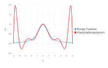
Interpolation of the Runge function with 11 equidistant support points (red points)

Does the interpolation quality improve when more interpolation points are added? Generally not: With equidistant support points and a high degree of the polynomial, it can happen that the polynomial function hardly resembles the function to be interpolated, which is also known as Runge's phenomenon . In the borderline case, polynomials tend towards . If the function to be interpolated behaves differently, e.g. periodically or asymptotically constant, strong oscillations occur near the interval limits. Polynomial interpolations over the entire interval are relatively unsuitable for such functions. ${\displaystyle x\to \pm \infty }$ ${\displaystyle \pm \infty }$

Chebyshev interpolation points, which are closer to the interval boundaries, can reduce the overall error of the interpolation, but a change in the interpolation method is recommended, for example to spline interpolation . Runge gave an example of this phenomenon, the Runge function named after him:

${\displaystyle f(x)={\frac {1}{1+x^{2}}}\,,\quad x\in [-5;5]}$

Convergence behavior

However, there are conditions under which the interpolation quality improves with an increasing number of interpolation points: When the interpolation point grid becomes more and more "finer" and an analytical function is interpolated. More precisely: Let be an analytic function on the interval . For an interval division ${\displaystyle f}$ ${\displaystyle I=[a,b]\subset \mathbb {R} }$

${\displaystyle \Delta _{m}=\{a=x_{0}^{(m)}<x_{1}^{(m)}<\dotsb <x_{n_{m}}^{(m)}=b\},\qquad m\in \mathbb {N} }$

let its norm be defined by

${\displaystyle \|\Delta _{m}\|=\max _{i}|x_{i+1}^{(m)}-x_{i}^{(m)}|.}$

For every interval division there is a clearly defined polynomial that interpolates at the interpolation points. If it holds for a sequence of interval divisions , then it follows uniformly . ${\displaystyle \Delta _{m}}$ ${\displaystyle P_{\Delta _{m}}}$ ${\displaystyle f}$ ${\displaystyle \Delta _{m}}$ ${\displaystyle \|\Delta _{m}\|\rightarrow 0}$ ${\displaystyle P_{\Delta _{m}}\rightarrow f}$

However, for every sequence a function that is continuous can also be found, so that it does not converge uniformly to ( Faber's theorem ). ${\displaystyle \{\Delta _{m}\}_{m\in \mathbb {N} }}$ ${\displaystyle I}$ ${\displaystyle f}$ ${\displaystyle \{P_{\Delta _{m}}\}_{m\in \mathbb {N} }}$ ${\displaystyle f}$

Best approximation

The relationship between the interpolation polynomial and the polynomial that best approximates the function with respect to the maximum norm is given as follows: ${\displaystyle \|\cdot \|_{\max }}$

Let the following objects be given

• a continuous function to be approximated: ${\displaystyle f\in C([a,b])}$
• Support points: ${\displaystyle x_{0},\ldots ,x_{n}\in [a,b]}$
• Lebesgue constant : ${\displaystyle \Lambda _{n}}$
• Interpolation polynomial: with ${\displaystyle P\in P_{n}}$ ${\displaystyle P(x_{i})=f(x_{i})}$
• Best approximation: with . ${\displaystyle Q\in P_{n}}$ ${\displaystyle \|f-Q\|_{\max }=\min _{R\in P_{n}}\|f-R\|_{\max }}$

Then the estimate applies

${\displaystyle \|f-P\|_{\max }=(1+\Lambda _{n})\|f-Q\|_{\max }\,.}$

generalization

So far, the interpolation points of the interpolation polynomial were assumed to be different in pairs. This is not the case with Hermit interpolation . Not only the function values ​​but also the values ​​of the derivatives of the interpolation polynomial are specified at interpolation points that occur multiple times. ${\displaystyle x_{i}}$ ${\displaystyle P}$

Lebesgue constant

Let the operator that assigns its interpolation polynomial to a function be defined by ${\displaystyle f}$ ${\displaystyle P(f)}$

${\displaystyle \phi _{n}\colon C([a,b])\rightarrow P_{n}\,,\,f\mapsto P(f)=\sum _{i=0}^{n}f(x_{i})l_{i}\,,}$

where the -th is Lagrange polynomial . ${\displaystyle l_{i}}$ ${\displaystyle i}$

As Lebesgue constant is operator norm of designated. For this, a standard is needed and often is here to the maximum norm accessed ${\displaystyle \Lambda _{n}}$ ${\displaystyle \phi _{n}}$ ${\displaystyle \|\cdot \|_{\max }}$

${\displaystyle \Lambda _{n}:=\|\phi _{n}\|_{\max }\,.}$

The norm can be evaluated explicitly

${\displaystyle \Lambda _{n}=\max _{x\in [a,b]}\sum _{i=0}^{n}|L_{i}(x)|\,.}$

literature

• Hans R. Schwarz, Norbert Köckler: Numerical Mathematics . 5th edition Teubner, Stuttgart 2004, ISBN 3-519-42960-8

• Stoer, Bulirsch: Numerical Mathematics 1 . 10th edition. Springer Verlag, Berlin, Heidelberg, New York 2007, ISBN 978-3-540-45389-5 , 2.1 Interpolation by Polynomials, pp. 39–57 (Covers Lagrange, Neville-Aitken, and Newton methods, Hermite interpolation, and error estimation, each with examples and evidence.).
• Press, Teukolsky, Vetterling, Flannery: Numerical Recipes . The Art of Scientific Computing. 3. Edition. Cambridge University Press, Cambridge 2007, ISBN 978-0-521-88407-5 , 3.2 Polynomial Interpolation and Extrapolation, pp. 118-120 (Neville-Aitken algorithm with C ++ implementation).
• Carl Runge: About empirical functions and the interpolation between equidistant ordinates . In: Journal of Mathematics and Physics . tape 46 . BG Teubner, Leipzig 1901, p. 224-243 ( hdl: 1908/2014 - Runge phenomenon).

Web links

Wikibooks: Divided Differences & Horner Scheme  - Implementations in the Algorithm Collection

• Newton, Lagrange and Cubic Spline page with Java applet
• Explanations and examples for Lagrange interpolation

Individual evidence

1. ^ Martin J. Marsden: An Identity for Spline Functions with Applications to Variation-Diminishing Spline Approximation . In: Journal of Approximation Theory , 3, 1970, pp. 7-49.
2. ↑ Jochen Werner: April 10 . In: Numerical Mathematics , 1st edition, Vieweg Studium, Nr.32, Vieweg Verlagsgesellschaft, 1992, ISBN 3-528-07232-6 . - 4.1.3. (PDF; 11.7 MB) sam.math.ethz.ch
3. ^ Andrei Nikolajewitsch Kolmogorow et al .: 4 . In: Mathematics of the 19th Century , 1st edition, Birkhäuser, 1998, ISBN 3-7643-5845-9 . - books.google.de