Unit root (time series analysis)

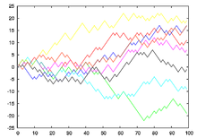
One speaks of a unit root in econometrics , especially in time series analysis , when 1 is a zero of the characteristic polynomial . A stochastic process that has such a root of unity is not stationary ; one also speaks of a stochastic trend . This is particularly important because many statistical estimation methods , such as the method of least squares , assume stationary data and give incorrect results if the underlying series are not stationary, as in the case of spurious regression .

Example AR (p) process

As an example, consider a discrete-time stochastic process { }. In addition, assume that this process can be represented as an autoregressive process of order p : ${\displaystyle y_{t},t=1,\infty }$ ${\displaystyle AR(p)}$

${\displaystyle y_{t}=a_{1}y_{t-1}+a_{2}y_{t-2}+\cdots +a_{p}y_{t-p}+\varepsilon _{t}}$

In this case { } is a non-autocorrelated stochastic process with the mean value zero and the constant variance . For the sake of simplicity, assume that . If a root of the characteristic polynomial ${\displaystyle \varepsilon _{t},t=0,\infty }$ ${\displaystyle \sigma ^{2}}$ ${\displaystyle y_{0}=0}$ ${\displaystyle m=1}$

${\displaystyle m^{p}-m^{p-1}a_{1}-m^{p-2}a_{2}-\cdots -a_{p}=0}$

is, then the stochastic process has a root of unity or, in other words, it is integrated with order 1, written . If there is a multiple zero of order , then the stochastic process is integrated with order . ${\displaystyle I(1)}$ ${\displaystyle m=1}$ ${\displaystyle r}$ ${\displaystyle I(r)}$

Example AR (1) process

A more specific example is the auto-regressive first order model : . This has a unity root, though . In this case is the characteristic polynomial . The solution to the equation is . If the process has a unit root, then the time series is nonstationary. That means the moments of the stochastic process depend on. It works out as follows. So in the case of a root of unity, the process is ${\displaystyle AR(1)}$ ${\displaystyle y_{t}=a_{1}y_{t-1}+\varepsilon _{t}}$ ${\displaystyle a_{1}=1}$ ${\displaystyle m-a_{1}=m-1}$ ${\displaystyle m=1}$ ${\displaystyle t}$

${\displaystyle y_{t}=y_{t-1}+\varepsilon _{t}}$

so that multiple substitution results. Hence the variance of ${\displaystyle y_{t}=\sum _{j=1}^{t}\varepsilon _{j}}$ ${\displaystyle y_{t}}$

${\displaystyle \operatorname {Var} (y_{t})=\sum _{j=1}^{t}\sigma ^{2}=t\sigma ^{2}}$

Because , however , the variance depends on. ${\displaystyle \operatorname {Var} (y_{1})=\sigma ^{2}}$ ${\displaystyle \operatorname {Var} (y_{2})=2\sigma ^{2}}$ ${\displaystyle t}$

If you differentiate a time series integrated with -th order , you get a stationary process. Optionally, there may be cointegration . ${\displaystyle n}$ ${\displaystyle n}$

Perception of processes with the roots of unity

Several realizations of a random walk starting in zero

William Feller indicates the probabilities of the proportion of time a random walk that starts in zero spends in the positive or negative numbers and uses this example to point out a possible misjudgment. The probability that predominantly positive or predominantly negative numbers are assumed is significantly greater than the probability of a balanced relationship: If, for example, the number of coats of arms and the number of numbers is noted when a coin is thrown twenty times, the probability is that over time either coat of arms or number at least 16 times in the lead is about 68.5%. In contrast, the probability that at the end the coat of arms and number were equally often in the lead is only about 6%. The intuitive assumption that a doubling of the observed time interval leads to a doubling of the crossings through zero is wrong.

See also

• Dickey-Fuller test

Individual evidence

1. ^ William Feller: An introduction to probability theory and its applications , second edition, Wiley, 1968, ISBN 0471257087 , p. 68. Hans Pécseli: Fluctuations in physical systems , Cambridge University Press, Cambridge 2000, ISBN 0521651921 , p. 87.