The Gauss quadrature (according to Carl Friedrich Gauß ) is a method for numerical integration that delivers an optimal approximation of the integral given a given degree of freedom. In this method, the function to be integrated is divided into , where is a weight function and is approximated by a special polynomial with specially selected evaluation points . This polynomial can be integrated exactly. So the procedure is of the form


-
 .
.
The weight function is greater than or equal to zero, has a finite number of zeros and can be integrated. is a continuous function . The integration range is not restricted to finite intervals. Furthermore, nodes, abscissa values or support points and the quantities are referred to as weights.
![[from]](https://wikimedia.org/api/rest_v1/media/math/render/svg/9c4b788fc5c637e26ee98b45f89a5c08c85f7935)

The method was published by Gauss in 1814, in its current form with orthogonal polynomials by Carl Gustav Jacobi in 1826.
properties
To achieve optimal accuracy, the abscissa values of a Gaussian quadrature formula of degree must correspond exactly to the zeros of the -th orthogonal polynomial of degree . The polynomials , ..., having to orthogonal with respect to the with weighted scalar product be


The following applies to the weights:

The Gaussian quadrature corresponds exactly to the value of the integral for polynomial functions whose degree is maximum . It can be shown that there is no quadrature formula that integrates all polynomials of degree exactly. In this regard, the order of the quadrature method is optimal.


Is the function to be integrated sufficiently smooth, i.e. H. it is times continuously differentiable in , so can the mistakes of Gaußquadratur with demonstrated support points:

-
 for a .
application
The Gaussian quadrature is used in numerical integration. For a given weight function and a given degree n, which determines the accuracy of the numerical integration, the support points and weight values are calculated and tabulated once . Subsequently, numerical integration can be carried out for any by simply adding up weighted function values.

This method is therefore potentially advantageous
- when many integrations have to be performed with the same weight function and
- if can be approximated sufficiently well by a polynomial.
For some special weight functions, the values for the support points and weights are completely tabulated.
Gauss-Legendre integration
This is the best known form of Gaussian integration on the interval , it is often simply referred to as Gaussian integration. It applies . The resulting orthogonal polynomials are the Legendre polynomials of the first kind. The case yields the midpoint rule . We get the approximation
with the support points and the associated weights![[-1.1]](https://wikimedia.org/api/rest_v1/media/math/render/svg/51e3b7f14a6f70e614728c583409a0b9a8b9de01)


-
 .
.
The extension to any intervals takes place through a variable transformation:
-
 .
.
The support points (also called Gauss points) and weights of the Gauss-Legendre integration are:
| n = 1
|
|
|
| 1 |
0 |
2
|
| n = 2
|
|
|
| 1 |
 |
1
|
| 2 |
 |
1
|
| n = 3
|
|
|
| 1 |
 |

|
| 2 |
0 |

|
| 3 |
 |
|
| n = 4
|
|
|
| 1 |
 |

|
| 2 |
 |

|
| 3 |
 |
|
| 4th |
 |
|
| n = 5
|
|
|
| 1 |
 |

|
| 2 |
 |

|
| 3 |
0 |

|
| 4th |
 |
|
| 5 |
 |
|
Gauss-Chebyshev integration
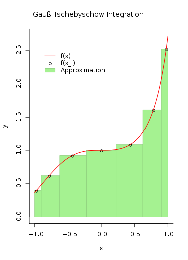
In contrast to the school method, the width of the individual bars, here called weight, is not constant, but decreases towards the edge of the interval. It amounts to .

A variant of the Gaussian integration on the interval is that with the weight function . The corresponding orthogonal polynomials are the Chebyshev polynomials , the zeros of which and thus also the support points of the quadrature formula are directly in analytical form:


while the weights only depend on the number of support points:
-
 .
.
The extension to any intervals is done by a variable transformation (see below). The integral you are looking for can be converted into . For the numerical calculation, the integral is now approximated by the sum . By inserting the support points in analytical form, one obtains


-
 ,
,
which corresponds to the n-fold application of the midpoint rule over the interval 0 to Pi. The error can be estimated for a suitable value for t between 0 and Pi using

Gauss-Hermite integration
Gaussian integration on the interval . It applies . The resulting orthogonal polynomials are the Hermite polynomials . The integral you are looking for can be converted into . For numerical calculation it is now approximated by the sum .


Support points and weights of the Gauß-Hermite integration:
| n = 1
|
|
|

|
| 1 |
0 |
 |
1.7724538509055159
|
| n = 2
|
|
|
|
| 1 |
 |
 |
1.46114118266
|
| 2 |
 |
|
1.46114118266
|
| n = 3
|
|
|
|
| 1 |
 |
 |
1.32393117521
|
| 2 |
0 |
 |
1.1816359006
|
| 3 |
 |
|
1.32393117521
|
| n = 4
|
|
|
|
| 1 |
−1.65068012389 |
0.0813128354472 |
1.2402258177
|
| 2 |
−0.524647623275 |
0.804914090006 |
1.05996448289
|
| 3 |
0.524647623275 |
0.804914090006 |
1.05996448289
|
| 4th |
1.65068012389 |
0.0813128354472 |
1.2402258177
|
Gauss-Laguerre integration
Gaussian integration on the interval . It applies . The resulting orthogonal polynomials are the Laguerre polynomials . The integral you are looking for can be converted into . For numerical calculation it is now approximated by the sum .


Support points and weights of the Gauss-Laguerre integration:
| n = 1
|
|
|

|
| 1 |
1 |
1 |
2.7182818284590451
|
| n = 2
|
|
|
|
| 1 |
 |
 |
1.53332603312
|
| 2 |
 |
 |
4,45095733505
|
| n = 3
|
|
|
|
| 1 |
0.415774556783 |
0.711093009929 |
1.07769285927
|
| 2 |
2.29428036028 |
0.278517733569 |
2.7621429619
|
| 3 |
6.28994508294 |
0.0103892565016 |
5.60109462543
|
| n = 4
|
|
|
|
| 1 |
0.322547689619 |
0.603154104342 |
0.832739123838
|
| 2 |
1.74576110116 |
0.357418692438 |
2.04810243845
|
| 3 |
4.53662029692 |
0.038887908515 |
3.63114630582
|
| 4th |
9.3950709123 |
0.000539294705561 |
6,48714508441
|
Gauss-Lobatto integration
This version, named after Rehuel Lobatto , integrates on the interval , with two of the support points at the ends of the interval. The weight function is . Polynomials up to the degree are precisely integrated.


Where , and to are the zeros of the first derivative of the Legendre polynomial . The weights are


With the tendon trapezoidal rule and with the Simpson rule .


| n |
Support points
|
Weights
|
 |
 |

|
 |
 |

|
|

|
 |
 |

|
|

|
 |
|

|
 |

|
|

|
 |
 |

|
 |

|
|

|
 |
|

|
 |

|
 |

|
|

|
Variable transformation in Gaussian quadrature
An integral over is reduced to an integral over before applying the Gaussian quadrature method. This transition can take place through
with and as well as and application of integration through substitution with in the following way:


Let the support points and the weights of the Gaussian quadrature be over the interval , or . Their connection is through


given.
Adaptive Gaussian method
Since the error in Gaussian quadrature, as mentioned above, depends on the number of selected support points and the denominator can increase significantly with a larger number of support points, this suggests that better approximations should be obtained with larger ones. The idea is to calculate a better approximation, for example , to an existing approximation in order to consider the difference between the two approximations. Provided that the estimated error a certain absolute requirement exceeds is to divide the interval so on and the can be done -Quadratur. However, the evaluation of a Gaussian quadrature is quite expensive, since new support points have to be calculated, especially for generally , so that the adaptive Gauss-Kronrod quadrature is suitable for the Gaussian quadrature with Legendre polynomials.


![\ left [a, {\ frac {a + b} {2}} \ right]](https://wikimedia.org/api/rest_v1/media/math/render/svg/2340575cf6aac755487555f6b71544a147ad4381)
![\ left [{\ frac {a + b} {2}}, b \ right]](https://wikimedia.org/api/rest_v1/media/math/render/svg/d5cd05ef535fe28124252885904819a07c058d8e)


Adaptive Gauss-Kronrod quadrature
The presented Kronrod modification, which only exists for the Gauss-Legendre quadrature, is based on the use of the already selected support points and the addition of new support points. While the existence of optimal extensions for the Gauss formulas was proven by Szegö, Kronrod (1965) derived optimal points for the Gauss-Legendre formulas that ensure the degree of precision . If the approximation calculated using the expanded nodal count of is defined as, the error estimate is:


This can then be compared with one in order to give the algorithm a termination criterion. The Kronrod knots and weights for the Gauss-Legendre knots and weights are recorded in the following table. The Gaussian nodes have been marked with a (G).


|
n = 3
|
|
|
| 1
|
~ 0.960491268708020283423507092629080
|
~ 0.104656226026467265193823857192073
|
| 2
|
~ 0.774596669241483377035853079956480 (G)
|
~ 0.268488089868333440728569280666710
|
| 3
|
~ 0.434243749346802558002071502844628
|
~ 0.401397414775962222905051818618432
|
| 4th
|
0 (G)
|
~ 0.450916538658474142345110087045571
|
| 5
|
~ -0.434243749346802558002071502844628
|
~ 0.401397414775962222905051818618432
|
| 6th
|
~ -0.774596669241483377035853079956480 (G)
|
~ 0.268488089868333440728569280666710
|
| 7th
|
~ -0.960491268708020283423507092629080
|
~ 0.104656226026467265193823857192073
|
|
n = 7
|
|
|
| 1
|
~ 0.991455371120812639206854697526329
|
~ 0.022935322010529224963732008058970
|
| 2
|
~ 0.949107912342758524526189684047851 (G)
|
~ 0.063092092629978553290700663189204
|
| 3
|
~ 0.864864423359769072789712788640926
|
~ 0.104790010322250183839876322541518
|
| 4th
|
~ 0.741531185599394439863864773280788 (G)
|
~ 0.140653259715525918745189590510238
|
| 5
|
~ 0.586087235467691130294144838258730
|
~ 0.169004726639267902826583426598550
|
| 6th
|
~ 0.405845151377397166906606412076961 (G)
|
~ 0.190350578064785409913256402421014
|
| 7th
|
~ 0.207784955007898467600689403773245
|
~ 0.204432940075298892414161999234649
|
| 8th
|
0 (G)
|
~ 0.209482141084727828012999174891714
|
| 9
|
~ -0.207784955007898467600689403773245
|
~ 0.204432940075298892414161999234649
|
| 10
|
~ -0.405845151377397166906606412076961 (G)
|
~ 0.190350578064785409913256402421014
|
| 11
|
~ -0.586087235467691130294144838258730
|
~ 0.169004726639267902826583426598550
|
| 12
|
~ -0.741531185599394439863864773280788 (G)
|
~ 0.140653259715525918745189590510238
|
| 13
|
~ -0.864864423359769072789712788640926
|
~ 0.104790010322250183839876322541518
|
| 14th
|
~ -0.949107912342758524526189684047851 (G)
|
~ 0.063092092629978553290700663189204
|
| 15th
|
~ -0.991455371120812639206854697526329
|
~ 0.022935322010529224963732008058970
|
Web links
literature
-
Philip J. Davis , Philip Rabinowitz: Methods of Numerical Integration. 2nd Edition. Academic Press, Orlando FL et al. 1984, ISBN 0-12-206360-0 .
- Vladimir Ivanovich Krylov: Approximate Calculation of Integrals. MacMillan, New York NY et al. 1962.
- Arthur H. Stroud, Don Secrest: Gaussian Quadrature Formulas. Prentice-Hall, Englewood Cliffs NJ 1966.
- Arthur H. Stroud: Approximate Calculation of Multiple Integrals. Prentice-Hall, Englewood Cliffs NJ 1971, ISBN 0-13-043893-6 .
swell
-
↑ Methodus nova integralium valores per approximationem inveniendi. In: Comm. Soc. Sci. Göttingen Math. Volume 3, 1815, pp. 29–76, Gallica , dated 1814, also in Werke, Volume 3, 1876, pp. 163–196.
-
^ CGJ Jacobi : About Gauss' new method to find the values of the integrals approximately. In: Journal for Pure and Applied Mathematics. Volume 1, 1826, pp. 301-308, (online) , and Werke, Volume 6.
-
↑
Ronald W. Freund, Ronald HW Hoppe: Stoer / Bulirsch: Numerische Mathematik 1 . Tenth, revised edition. Springer-Verlag, Berlin / Heidelberg 2007, p. 195.
-
↑ a b
Robert Piessens, Elise de Doncker-Kapenga, Christoph W. About Huber, David K. Kahaner: QUADPACK: A subrotine package for automatic integration. Springer-Verlag, Berlin / Heidelberg / New York 1983, pp. 16-17.

