Gozintograph

This article or the following section is not adequately provided with supporting documents ( e.g. individual evidence ). Information without sufficient evidence could be removed soon. Please help Wikipedia by researching the information and including good evidence.

The gozintograph (also gozinto graph ) is a directed graph that describes the parts of one or more products. The production process can be multi-stage, with the input consisting of raw materials , semi- finished and finished parts . The gozintograph shows how these parts are possibly quantitatively interwoven. The nodes designate the parts and the directed edges indicate how many units of a part flow into a unit of a downstream part.

The name of this graph is a joking corruption : the mathematician Andrew Vazsonyi named the fictional Italian mathematician Zepartzat Gozinto as the author in 1962 , which means nothing other than the part that goes into . This term is now generally accepted.

The gozintograph is mainly used in the area of production planning and control for the resolution of parts lists . The contents of the graph can be incorporated into a linear system of equations . This then usually results in very large, sparsely populated coefficient matrices which, depending on the structure, enable different solution methods.

example

In the following simplified example, 200 extension cables, 100 plugs and 50 sockets are to be produced for a DIY store. The end products are made up of different parts, pins, screws, clamps, inner parts, covers, etc. The following table lists the individual parts:

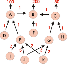
Gozintograph for creating electrical items

symbol	index	part
A.	1	plug
B.	2	extension cable
C.	3	socket
D.	4th	Cover set connector
E.	5	Body connector
F.	6th	electric wire
G	7th	Body box
H	8th	Lid set can
I.	9	pen
J	10	screw
K	11	clamp

The interrelationships can be converted into a system of equations. First, the gozintograph shows how many units of each part are needed.

${\displaystyle A=100+1\cdot {B}}$	${\displaystyle B=200\,\!}$	${\displaystyle C=50+1\cdot {B}}$	${\displaystyle D=1\cdot {A}}$	${\displaystyle E=1\cdot {A}}$	${\displaystyle F=1\cdot {B}}$
${\displaystyle G=1\cdot {C}}$	${\displaystyle H=1\cdot {C}}$	${\displaystyle I=2\cdot {E}}$	${\displaystyle J=5\cdot {E}+3\cdot {G}}$	${\displaystyle K=2\cdot {E}+2\cdot {G}}$

version 1

Due to the simple structure of this example, the individual equations can be solved successively. It is required:

${\displaystyle A=300}$	${\displaystyle B=200}$	${\displaystyle C=250}$	${\displaystyle D=300}$	${\displaystyle E=300}$	${\displaystyle F=200}$
${\displaystyle G=250}$	${\displaystyle H=250}$	${\displaystyle I=600}$	${\displaystyle J=2{.}250}$	${\displaystyle K=1{.}100}$

To create a coefficient matrix for the system of equations, the equations are converted accordingly, e.g. B .:

${\displaystyle 1\,A=100+1\,B\Leftrightarrow {1\,A-1\,B=100}}$

The coefficients of this linear system of equations then form the so-called technology matrix T :

${\displaystyle {\begin{array}{|ccccccccccc|}1&-1&\color {Gray}{0}&\color {Gray}{0}&\color {Gray}{0}&\color {Gray}{0}&\color {Gray}{0}&\color {Gray}{0}&\color {Gray}{0}&\color {Gray}{0}&\color {Gray}{0}\\\color {Gray}{0}&1&\color {Gray}{0}&\color {Gray}{0}&\color {Gray}{0}&\color {Gray}{0}&\color {Gray}{0}&\color {Gray}{0}&\color {Gray}{0}&\color {Gray}{0}&\color {Gray}{0}\\\color {Gray}{0}&-1&1&\color {Gray}{0}&\color {Gray}{0}&\color {Gray}{0}&\color {Gray}{0}&\color {Gray}{0}&\color {Gray}{0}&\color {Gray}{0}&\color {Gray}{0}\\-1&\color {Gray}{0}&\color {Gray}{0}&1&\color {Gray}{0}&\color {Gray}{0}&\color {Gray}{0}&\color {Gray}{0}&\color {Gray}{0}&\color {Gray}{0}&\color {Gray}{0}\\-1&\color {Gray}{0}&\color {Gray}{0}&\color {Gray}{0}&1&\color {Gray}{0}&\color {Gray}{0}&\color {Gray}{0}&\color {Gray}{0}&\color {Gray}{0}&\color {Gray}{0}\\\color {Gray}{0}&-1&\color {Gray}{0}&\color {Gray}{0}&\color {Gray}{0}&1&\color {Gray}{0}&\color {Gray}{0}&\color {Gray}{0}&\color {Gray}{0}&\color {Gray}{0}\\\color {Gray}{0}&\color {Gray}{0}&-1&\color {Gray}{0}&\color {Gray}{0}&\color {Gray}{0}&1&\color {Gray}{0}&\color {Gray}{0}&\color {Gray}{0}&\color {Gray}{0}\\\color {Gray}{0}&\color {Gray}{0}&-1&\color {Gray}{0}&\color {Gray}{0}&\color {Gray}{0}&\color {Gray}{0}&1&\color {Gray}{0}&\color {Gray}{0}&\color {Gray}{0}\\\color {Gray}{0}&\color {Gray}{0}&\color {Gray}{0}&\color {Gray}{0}&-2&\color {Gray}{0}&\color {Gray}{0}&\color {Gray}{0}&1&\color {Gray}{0}&\color {Gray}{0}\\\color {Gray}{0}&\color {Gray}{0}&\color {Gray}{0}&\color {Gray}{0}&-5&\color {Gray}{0}&-3&\color {Gray}{0}&\color {Gray}{0}&1&\color {Gray}{0}\\\color {Gray}{0}&\color {Gray}{0}&\color {Gray}{0}&\color {Gray}{0}&-2&\color {Gray}{0}&-2&\color {Gray}{0}&\color {Gray}{0}&\color {Gray}{0}&1\end{array}}\cdot {\begin{array}{|c|}A\\B\\C\\D\\E\\F\\G\\H\\I\\J\\K\end{array}}={\begin{array}{|c|}100\\200\\50\\\color {Gray}{0}\\\color {Gray}{0}\\\color {Gray}{0}\\\color {Gray}{0}\\\color {Gray}{0}\\\color {Gray}{0}\\\color {Gray}{0}\\\color {Gray}{0}\end{array}}}$

or in matrix notation:

${\displaystyle \mathbf {T} \cdot {\vec {g}}={\vec {p}}}$

The column vector represents the so-called primary requirement . Its components are the specifications for the sales quantities and / or the planned inventory build-up of the components i. In the above example , , , all others are 0. The column vector is the total demand (independent requirements plus derived demand) for this production. ${\displaystyle {\vec {p}}}$ ${\displaystyle p_{i}}$ ${\displaystyle p_{1}=100}$ ${\displaystyle p_{2}=200}$ ${\displaystyle p_{3}=50}$ ${\displaystyle p_{i}}$ ${\displaystyle {\vec {g}}}$

Variant 2

Alternatively, the so-called direct demand matrix D can be drawn up directly from the gozintograph : The values ​​of the matrix elements are the numbers that are in the gozintograph on the arrow leading from component i to component j. All those for whom there is no arrow in the gozintograph receive the value zero. In other words: is the number of components i that end up in component j. D is therefore of type n × n if the Gozintograph has n nodes. In the example, n = 11. From a purely mathematical point of view, the direct demand matrix is ​​therefore nothing other than the weight matrix of the respective gozintograph. ${\displaystyle D_{i,j}}$ ${\displaystyle D_{i,j}}$ ${\displaystyle D_{i,j}}$

${\displaystyle \mathbf {D} ={\begin{array}{|ccccccccccc|}\color {Gray}{0}&1&\color {Gray}{0}&\color {Gray}{0}&\color {Gray}{0}&\color {Gray}{0}&\color {Gray}{0}&\color {Gray}{0}&\color {Gray}{0}&\color {Gray}{0}&\color {Gray}{0}\\\color {Gray}{0}&\color {Gray}{0}&\color {Gray}{0}&\color {Gray}{0}&\color {Gray}{0}&\color {Gray}{0}&\color {Gray}{0}&\color {Gray}{0}&\color {Gray}{0}&\color {Gray}{0}&\color {Gray}{0}\\\color {Gray}{0}&1&\color {Gray}{0}&\color {Gray}{0}&\color {Gray}{0}&\color {Gray}{0}&\color {Gray}{0}&\color {Gray}{0}&\color {Gray}{0}&\color {Gray}{0}&\color {Gray}{0}\\1&\color {Gray}{0}&\color {Gray}{0}&\color {Gray}{0}&\color {Gray}{0}&\color {Gray}{0}&\color {Gray}{0}&\color {Gray}{0}&\color {Gray}{0}&\color {Gray}{0}&\color {Gray}{0}\\1&\color {Gray}{0}&\color {Gray}{0}&\color {Gray}{0}&\color {Gray}{0}&\color {Gray}{0}&\color {Gray}{0}&\color {Gray}{0}&\color {Gray}{0}&\color {Gray}{0}&\color {Gray}{0}\\\color {Gray}{0}&1&\color {Gray}{0}&\color {Gray}{0}&\color {Gray}{0}&\color {Gray}{0}&\color {Gray}{0}&\color {Gray}{0}&\color {Gray}{0}&\color {Gray}{0}&\color {Gray}{0}\\\color {Gray}{0}&\color {Gray}{0}&1&\color {Gray}{0}&\color {Gray}{0}&\color {Gray}{0}&\color {Gray}{0}&\color {Gray}{0}&\color {Gray}{0}&\color {Gray}{0}&\color {Gray}{0}\\\color {Gray}{0}&\color {Gray}{0}&1&\color {Gray}{0}&\color {Gray}{0}&\color {Gray}{0}&\color {Gray}{0}&\color {Gray}{0}&\color {Gray}{0}&\color {Gray}{0}&\color {Gray}{0}\\\color {Gray}{0}&\color {Gray}{0}&\color {Gray}{0}&\color {Gray}{0}&2&\color {Gray}{0}&\color {Gray}{0}&\color {Gray}{0}&\color {Gray}{0}&\color {Gray}{0}&\color {Gray}{0}\\\color {Gray}{0}&\color {Gray}{0}&\color {Gray}{0}&\color {Gray}{0}&5&\color {Gray}{0}&3&\color {Gray}{0}&\color {Gray}{0}&\color {Gray}{0}&\color {Gray}{0}\\\color {Gray}{0}&\color {Gray}{0}&\color {Gray}{0}&\color {Gray}{0}&2&\color {Gray}{0}&2&\color {Gray}{0}&\color {Gray}{0}&\color {Gray}{0}&\color {Gray}{0}\end{array}}}$

The columns of D that belong to raw materials (purchased parts) j therefore contain only zeros, as do the rows of D that belong to end products i that are not used for the manufacture of other components. If again the independent demand and the derived demand arising for the production of the independent demand (its components are the quantities of all semi-finished products and raw materials required to cover the independent demand ), then the total demand vector is defined as: ${\displaystyle {\vec {p}}}$ ${\displaystyle {\vec {a}}}$ ${\displaystyle a_{i}}$ ${\displaystyle {\vec {g}}}$

(1)   ${\displaystyle {\vec {g}}={\vec {p}}+{\vec {a}}}$

The example is easy to convince yourself that

(2)   ${\displaystyle \mathbf {D} \cdot {\vec {g}}={\vec {a}}}$

From (1) and (2) it follows again

(3)   ${\displaystyle \mathbf {(E-D)} \cdot {\vec {g}}=\mathbf {T} \cdot {\vec {g}}={\vec {p}}}$

where E is the identity matrix of dimension n and (E - D) = T, the technology matrix from variant 1.

application

By inversion of the technology matrix T set up according to variant 1 or 2, (3) can be resolved according to : ${\displaystyle {\vec {g}}}$

${\displaystyle {\vec {g}}=\mathbf {(E-D)^{-1}} \cdot {\vec {p}}=\mathbf {T^{-1}} \cdot {\vec {p}}}$

For our example we get : ${\displaystyle (E-D)^{-1}}$

${\displaystyle {\begin{array}{|ccccccccccc|}1&1&\color {Gray}{0}&\color {Gray}{0}&\color {Gray}{0}&\color {Gray}{0}&\color {Gray}{0}&\color {Gray}{0}&\color {Gray}{0}&\color {Gray}{0}&\color {Gray}{0}\\\color {Gray}{0}&1&\color {Gray}{0}&\color {Gray}{0}&\color {Gray}{0}&\color {Gray}{0}&\color {Gray}{0}&\color {Gray}{0}&\color {Gray}{0}&\color {Gray}{0}&\color {Gray}{0}\\\color {Gray}{0}&1&1&\color {Gray}{0}&\color {Gray}{0}&\color {Gray}{0}&\color {Gray}{0}&\color {Gray}{0}&\color {Gray}{0}&\color {Gray}{0}&\color {Gray}{0}\\1&1&\color {Gray}{0}&1&\color {Gray}{0}&\color {Gray}{0}&\color {Gray}{0}&\color {Gray}{0}&\color {Gray}{0}&\color {Gray}{0}&\color {Gray}{0}\\1&1&\color {Gray}{0}&\color {Gray}{0}&1&\color {Gray}{0}&\color {Gray}{0}&\color {Gray}{0}&\color {Gray}{0}&\color {Gray}{0}&\color {Gray}{0}\\\color {Gray}{0}&1&\color {Gray}{0}&\color {Gray}{0}&\color {Gray}{0}&1&\color {Gray}{0}&\color {Gray}{0}&\color {Gray}{0}&\color {Gray}{0}&\color {Gray}{0}\\\color {Gray}{0}&1&1&\color {Gray}{0}&\color {Gray}{0}&\color {Gray}{0}&1&\color {Gray}{0}&\color {Gray}{0}&\color {Gray}{0}&\color {Gray}{0}\\\color {Gray}{0}&1&1&\color {Gray}{0}&\color {Gray}{0}&\color {Gray}{0}&\color {Gray}{0}&1&\color {Gray}{0}&\color {Gray}{0}&\color {Gray}{0}\\2&2&\color {Gray}{0}&\color {Gray}{0}&2&\color {Gray}{0}&\color {Gray}{0}&\color {Gray}{0}&1&\color {Gray}{0}&\color {Gray}{0}\\5&8&3&\color {Gray}{0}&5&\color {Gray}{0}&3&\color {Gray}{0}&\color {Gray}{0}&1&\color {Gray}{0}\\2&4&2&\color {Gray}{0}&2&\color {Gray}{0}&2&\color {Gray}{0}&\color {Gray}{0}&\color {Gray}{0}&1\end{array}}}$

This enables the total requirement for a given primary requirement and, using (1), the derived requirement to be calculated. The matrix is therefore also known as total demand matrix G called. By additionally taking existing stocks into account, one can then calculate back from the gross requirement considered here to the net requirement. ${\displaystyle {\vec {p}}}$ ${\displaystyle {\vec {g}}}$ ${\displaystyle {\vec {a}}}$ ${\displaystyle (E-D)^{-1}}$

Individual evidence

1. ^ Heiner Müller-Merbach: data organization . 2nd, improved edition. Walter de Gruyter, Berlin / New York 1972, ISBN 3-11-004151-0 . - Here he refers to A. Vazsonyi: The planning calculation in economy and industry (German translation). Vienna / Munich 1962
   Heiner Müller-Merbach: Operations Research . 3. Edition. Verlag Franz Vahlen, Munich 1973, ISBN 3-8006-0388-8 , p. 259