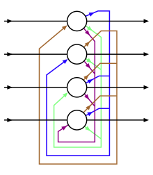
Hopfield network

This article or the following section is not adequately provided with supporting documents ( e.g. individual evidence ). Information without sufficient evidence could be removed soon. Please help Wikipedia by researching the information and including good evidence.

Not a single proof. For example, the work of Hopfield should be linked. - Martin Thoma 1:42 p.m., Dec. 6, 2015 (CET)

Hopfield network with four "neurons"

A special form of an artificial neural network is called a Hopfield network . It is named after the American scientist John Hopfield who made the model popular in 1982.

structure

Hopfield networks belong to the class of feedback networks (networks with feedback ). In a Hopfield network, there is only one layer that simultaneously functions as an input and output layer. Each of the McCulloch-Pitts binary neurons is connected to everyone except themselves. The neurons can assume the values ​​−1 and 1, which correspond to the states “does not fire” and “fires”.

In Hopfield networks, the synaptic weights are symmetrical ; H. it applies to all i and j . Although this does not make sense from a biological point of view, it allows an energy function to be set up and the networks to be analyzed using methods of statistical mechanics . ${\displaystyle w_{i,j}=w_{j,i}}$

Since the same artificial neurons are used for input and output, it is also called an auto-association network .

Working method

When implementing a Hopfield network, the question arises whether the weights of the neurons should be changed synchronously or asynchronously.

• synchronous change means that all neurons are updated at the same time in one iteration step.

• Asynchronous change means that a neuron is randomly selected and calculated and the value is immediately taken into account in the next calculation.

Asynchronous changing of the Hopfield network is the most common.

Pattern recovery with Hopfield networks

Hopfield networks can be used as auto-associative memory to reconstruct noisy or only partially existing patterns. This happens in three phases:

Training phase

Here a number L of predetermined patterns are stored in the network. This is done by adjusting the synaptic weights. We are looking for a suitable symmetrical weight matrix of size . For example, it can be calculated in one step using the following rule, which is also known as the generalized Hebbian learning rule : ${\displaystyle N\times N}$

${\displaystyle w_{i,j}=w_{j,i}={\begin{cases}\sum \limits _{\mu =1}^{L}M_{\mu i}\cdot M_{\mu j}{\text{,}}&{\text{falls }}i\neq j\\0&{\text{sonst,}}\end{cases}}}$

in which

${\displaystyle L}$ the number of patterns to be associated,

${\displaystyle N}$ the number of dimensions of a pattern and

${\displaystyle M\in \mathbb {R} ^{L\times N}}$ denote the (unsupervised) learning task

In general, one would like to feed as many different patterns as possible into a Hopfield. However, the storage capacity is limited according to the ratio . ${\displaystyle {\tfrac {L}{N}}}$

Entering a test pattern

Now you put a test pattern, for example a noisy or incomplete image into the network. To do this, you simply put the neurons in the state that corresponds to the test pattern.

Calculation phase

The neurons are updated asynchronously with the following rule:

${\displaystyle s_{i}=\left\{{\begin{array}{ll}1&{\text{wenn }}\sum _{j}{w_{ij}s_{j}}>\theta _{i},\\-1&{\text{sonst,}}\end{array}}\right.}$

where is the state of the neuron to be updated and a threshold. ${\displaystyle s_{i}}$ ${\displaystyle \theta _{i}}$

In this case, the result could be an image with more or less noise reduction depending on the number of iteration steps. Up to a ratio (ratio of patterns to be stored to neurons of the Hopfield network), Hebb's rule guarantees that the system will no longer change when it has reached a state that corresponds to one of the stored patterns. It can also be shown that the system always arrives in a stable final state. ${\displaystyle {\tfrac {L}{N}}=0{,}138}$

The following three final states are conceivable:

• The pattern was recognized correctly.
• The inverted pattern was recognized.
• No pattern can be recognized, the network enters a stable spurious state that does not correspond to any of the patterns.

Relationship to statistical mechanics

For the Hopfield model there is an energy function of the form

${\displaystyle E=-{\frac {1}{2}}\sum _{i\neq j}{w_{ij}{s_{i}}{s_{j}}}+\sum _{i}{\theta _{i}s_{i}}}$,

the value of which, as can be proven, decreases with each update according to the above rule. Only in the case of the stable patterns (and the inauthentic states) does the energy remain the same, so these represent local minima of the energy landscape.

There is a connection between the Hopfield model and the Ising model , for whose energy the following applies:

${\displaystyle E=-{\frac {1}{2}}\sum _{\langle ij\rangle }{J_{ij}{s_{i}}{s_{j}}}+\sum _{i}{h_{i}s_{i}}}$.

In particular , there is great similarity to spin glasses , where they are randomly distributed. So it could be shown with methods of theoretical physics that Hopfield networks can only be used as associative memory up to a certain ratio . ${\displaystyle J_{ij}}$ ${\displaystyle {\tfrac {L}{N}}=0{,}138}$

Web links

• Convergence of the discrete Hopfield network (PDF; 70 kB)
• Hopfield Network . In: Scholarpedia . (English, including references)

Individual evidence

1. ^ ^{A b} Rudolf Kruse et al .: Computational Intelligence: A methodical introduction to Artificial Neural Networks, Evolutionary Algorithms, Fuzzy Systems and Bayesian Networks. Second edition. Springer-Vieweg, Wiesbaden 2015, ISBN 978-3-658-10903-5 , pp. 515 .
2. ↑ ^{a b} Rudolf Kruse et al .: Neural Networks | Computational Intelligence. In: Computational Intelligence: A methodical introduction to Artificial Neural Networks, Evolutionary Algorithms, Fuzzy Systems and Bayesian Networks. Second edition. Springer-Vieweg, Wiesbaden, 2015, accessed on April 5, 2017 .