Difference equation

This item has been on the quality assurance side of the portal mathematics entered. This is done in order to bring the quality of the mathematics articles to an acceptable level . Please help fix the shortcomings in this article and please join the discussion !  ( Enter article )

A difference equation is a recursive calculation rule for a discrete sequence of values ​​separated by an interval . Each calculated follow-up member refers to a previous follow-up member or several previous follow-up members, depending on the order of the difference equation. ${\displaystyle y_{k},\,k=(0,\ 1,\ 2,\ 3,\dotsc )}$ ${\displaystyle \Delta x}$

Difference equations are used for numerical calculation in many scientific disciplines - such as economics, medicine, technology, electrical engineering, cybernetics, computer science, acoustics and others - whose problems can be described by ordinary or partial differential equations.

definition

In mathematics , an equation is of form

${\displaystyle y_{k+n}=f(k,y_{k+n-1},y_{k+n-2},\dotsc ,y_{k}),k=0,1,2,\dotsc }$

referred to as the difference equation or recursion equation of order . The linear difference equations are a special form . ${\displaystyle n}$

An implicit difference equation is present if it cannot be solved for the term with the highest order:

${\displaystyle y_{k+n}=f(k,y_{k+n},y_{k+n-1},y_{k+n-2},\dotsc ,y_{k}),k=0,1,2,\dotsc }$

The simplest method for creating the difference equations is the explicit Euler segment method . Other methods of numerical calculation are used for a better approximation z. B. instead of the Euler stretching method , the trapezoidal surface method ( Heun method ), the multi-step method (Adams-Bashforth method) and other methods.

Applications

Differential equations are used in many fields to describe dynamic systems. Their numerical solution is done using difference equations. Examples are:

• Weather simulation ( finite difference method )
• Trajectory tracking of satellites ( space flight mechanics ).
• Control technology : The best-known programs such as Matlab and Simulink with extensive instruction sets for the theoretical modeling of dynamic systems and many special cybernetic and control applications are available for the engineering sector . The simulations can be carried out offline or in real time .
• Multi-body simulation
• Epidemiology ( SIR model )
• Economy or Biology ( Lotka-Volterra equations )

Difference equations according to the Euler route train method

In general, a difference equation of the order gradually calculates a sequence of values with the following terms in the interval . The first members are the initial values. ${\displaystyle n}$ ${\displaystyle y_{k+n}}$ ${\displaystyle k=(0,1,2,3,\dotsc ,k_{\text{max}})}$ ${\displaystyle h=\Delta x}$ ${\displaystyle n}$

Since ordinary differential equations of a higher order can be converted into individual differential equations of the first order, order 1 can be assumed for further considerations. In the simplest integration method, first order difference equations are formed from this. With the initial value , the next interpolation point can be calculated using the difference equation . This also applies to all other support points. ${\displaystyle y(x_{0})=y_{0}}$ ${\displaystyle y_{1}}$ ${\displaystyle x_{1}}$

Higher-order linear systems, which are broken down into first-order differential equations and whose system behavior is calculated using first-order difference equations, converge to the exact solution according to the Euler method when the interval or, in the time domain, the interval approaches zero. ${\displaystyle h}$ ${\displaystyle \Delta t}$

Explicit Euler route method (Euler forward)

See also : Explicit Euler Method

The simplest method for solving first-order differential equations is the explicit Euler method.

For each calculation step (support point, node), the derivative is approximated by a forward difference quotient. The term forward difference quotient refers to the left interval limit. ${\displaystyle y'(x)}$

The forward difference quotient for a differential equation and the step size is: ${\displaystyle y'=f(x,y)}$ ${\displaystyle h}$

${\displaystyle y'\approx {\frac {\Delta y}{\Delta x}}={\frac {y(x+h)-y(x)}{(x+h)-x}}:={\frac {y_{k+1}-y_{k}}{h}}}$

In the Euler forward method, the integral for a segment is approximated:

${\displaystyle \int _{x}^{x+h}f(y(x))dx\approx h\cdot f(y_{k},x_{k})}$

The approximation for the integral is the stipulation that the integrand is constant in the entire integration interval and can be replaced by the value at the left edge of the integration interval. ${\displaystyle f(x,y)}$ ${\displaystyle f(x,y)}$

The algorithm for approximating the integral leads to the following calculation rule:

${\displaystyle y_{k+1}=y_{k}+h\cdot f(y_{k},x_{k})}$

It means:

• ${\displaystyle {y_{k+1}}}$= ${\displaystyle {\begin{bmatrix}y_{0}&=&y_{0}\\y_{1}&=&y_{0}&+&\ h\cdot f(y_{0},x_{0})\\y_{2}&=&y_{1}&+&\ h\cdot f(y_{1},x_{1})\\y_{k+1}&=&y_{k}&+&\ h\cdot f(y_{k},x_{k})\\\end{bmatrix}}}$

${\displaystyle {y_{k+1}}}$is the new value of the recursive difference equation. is assigned to the initial value. ${\displaystyle {y_{k=0}}}$

The explicit Euler method is also referred to under the term: integration formula ( Euler-Cauchy method).

Implicit Euler route train method (Euler backward)

→ Main article : Implicit Euler method

The implicit Euler method arises when, when the integral is approximated by a rectangular area, the function value is evaluated not at the left but at the right edge of the interval:

${\displaystyle \int _{x}^{x+h}f(y(x))dx\approx h\cdot f(y_{k+1},x_{k+1})}$

This leads to the following implicit calculation rule:

${\displaystyle y_{k+1}=y_{k}+h\cdot f(y_{k+1},x_{k+1})}$

Remarks:

• The implicit Euler method depends on itself. Either an iteration or a predictor step is therefore required to compute . This problem does not exist with linear systems, since after can be resolved. ${\displaystyle y_{k+1}}$ ${\displaystyle y_{k+1}}$ ${\displaystyle y_{k+1}}$
• The implicit Euler route train method is the more stable method than the explicit method. It is therefore z. B. used in rigid differential equations that arise in applications in hydraulics.

Simple one-variable difference equations

A difference equation is a discrete calculation rule for the terms of a recursively defined sequence. It contains values ​​of a variable at different points in time. The next following element is calculated from one element of the sequence. An initial value is always required to calculate the following elements . ${\displaystyle y_{k}}$ ${\displaystyle y_{k}=y_{0}}$

This section is not an approximation to a course of a mathematical function given by differential equations, but the difference equations shown below result from the task. A distinction is made between the following elements:

• In the arithmetic sequence, each follow-up member increases or decreases by a fixed amount.
• In the case of the exponential sequence, each subsequent member increases or decreases by a relative proportion.

Example: Given a homogeneous difference equation with the following notation:

${\displaystyle \Delta y_{k}-0{,}5\cdot y_{k}=0\quad |\quad {\text{mit}}\quad \Delta y_{k}=y_{k+1}-y_{k}}$

After rearranging the equations, this equation can be represented equally in various forms:

• ${\displaystyle y_{k+1}-y_{k}-0{,}5\cdot y_{k}=0\quad |\quad \Delta y_{k}=y_{k+1}-y_{k}\ {\text{eingesetzt}}}$
• ${\displaystyle y_{k+1}-1{,}5\cdot y_{k}=0}$
• ${\displaystyle y_{k+1}=1{,}5\cdot y_{k}}$

This form of the difference equation is often used for simple tasks such as compound interest calculation, temporal development of the population, slowed growth, warming up or cooling down liquids, emptying containers (without friction) and others. The calculation of these tasks is exact and can be carried out for the sequence by calculating the individual follow-up elements in a table . ${\displaystyle k=(0,\ 1,\ 2,\dotsc ,\ k_{\text{kmax}})}$

For the exponential sequence, an equation can be created with the so-called growth factor as the basis for an exponential function, which allows the calculation of individual sequences for any one . ${\displaystyle y_{k}}$ ${\displaystyle k}$

Example of calculating a sequence:

The following terms are determined from the first order difference equation:

${\displaystyle y_{k+1}=1{,}5\cdot y_{k}}$.

Sequence with the initial value : ${\displaystyle y_{0}=4}$

${\displaystyle y_{0}=4}$

${\displaystyle y_{1}=1{,}5\cdot y_{0}=1{,}5\cdot 4=6}$

${\displaystyle y_{2}=1{,}5\cdot y_{1}=1{,}5\cdot 6=9}$

${\displaystyle y_{3}=1{,}5\cdot y_{2}=1{,}5\cdot 9=13{,}5}$

The difference between the calculated successor elements is not constant. The values ​​of the following members take an exponential course. The calculation of further following elements can be done in this way for any values ​​from tabular. ${\displaystyle y_{k+1}-y_{k}}$ ${\displaystyle y_{k}}$ ${\displaystyle k}$

From this simple difference equation with the help of the subsequent members and the formation law for any numbered subsequent member can be guessed and formed. For this application, the factor vor applies as the basis of the exponential function and is referred to as the growth factor. ${\displaystyle y_{1}=1{,}5\cdot y_{0}}$ ${\displaystyle y_{2}=1{,}5\cdot y_{1}}$ ${\displaystyle y_{k}=1{,}5}$

${\displaystyle y_{k}=1{,}5^{k}\cdot y_{0}}$

Example of a difference equation for numerically calculating population growth

Example of population growth over 50 years as a function of the birth rate and the death rate

Given: The population of a state at the beginning: millions ${\displaystyle B_{0}=20}$ Constant birth rate: per year ${\displaystyle G=6\ \%}$ Constant death rate: per year ${\displaystyle S=2\ \%}$ The increment is year ${\displaystyle h=1}$ Wanted: population development after 50 years Wanted: Difference equation to determine population growth Starting value: Millions at the beginning of the first year ${\displaystyle B_{0}=20}$ Adjusted birth rate: ${\displaystyle a=G-S=(6-2)\ \%{\text{ pro Jahr}}=4\ \%{\text{ pro Jahr}}}$ Difference equation: ${\displaystyle B_{k+1}=B_{k}+B_{k}\cdot a\cdot h=B_{k}+B_{k}\cdot {\frac {0{,}04}{1\ \mathrm {Jahr} }}\cdot 1\ \mathrm {Jahr} =B_{k}+B_{k}\cdot 0{,}04}$ Development of the following links: Year k + 1 ${\displaystyle B_{k}+B_{k}\cdot 0{,}04}$ in millions Population in millions ${\displaystyle B_{k+1}}$ 1 ${\displaystyle 20+20\cdot 0{,}04}$ ${\displaystyle 20\cdot 1{,}04^{1}=20{,}8}$ 2 ${\displaystyle 20{,}8+20{,}8\cdot 0{,}04}$ ${\displaystyle 20\cdot 1{,}04^{2}=21{,}632}$ 3 ${\displaystyle 21{,}632+21{,}632\cdot 0{,}04}$ ${\displaystyle 20\cdot 1{,}04^{3}=22{,}49728}$ ${\displaystyle \vdots }$ ${\displaystyle \vdots }$ ${\displaystyle \vdots }$ 50 ${\displaystyle 20\cdot 1{,}04^{49}+20\cdot 1{,}04^{49}\cdot 0{,}04}$ ${\displaystyle 20\cdot 1{,}04^{50}\approx 142}$ ${\displaystyle B_{k+1}=B_{k}+B_{k}\cdot 0{,}04=B_{k}\cdot 1{,}04=B_{0}\cdot 1{,}04^{k+1}=20\cdot 1{,}04^{k+1}}$ ${\displaystyle 1{,}04}$ is the growth factor here. The results of the subsequent equations give support points with exponential growth.

Note: Unrestrained growth calculated with this linear difference equation will not exist in practice because other influences such as B. Food shortages counteract this.

Example of a numerical calculation of the capital development with compound interest

Model: difference equations of the type ${\displaystyle y_{k+1}=f(y_{k})}$

The compound interest calculation is a constant increase in annual interest based on the current amount saved in a sequence. The capital development from the initial capital over the following years takes a progressive course.

Given: Initial value = € = capital at the beginning ${\displaystyle K_{0}=1000}$ Rate of interest = ${\displaystyle p=2}$ Interest rate = per year (at the end of the year) ${\displaystyle i=2\ \%}$ Duration = years ${\displaystyle L=20}$ Increment = year ${\displaystyle h=1}$ Wanted: difference equation, final capital Difference equation: ${\displaystyle K_{k+1}=K_{k}+K_{k}\cdot i\cdot h}$ Growth factor : ${\displaystyle q={\frac {K_{k+1}}{K_{k}}}=\left(1+{\frac {p}{100}}\right)=1{,}02}$ Tabular development of the following members : ${\displaystyle k=0,1,2,\dots 19}$ year Capital at the beginning of the year in € ${\displaystyle K_{k}\cdot 1{,}02}$ in € Capital at the end of the year in € 1 ${\displaystyle 1000}$ ${\displaystyle 1000\cdot 1{,}02}$ ${\displaystyle 1000\cdot 1{,}02=1020}$ 2 ${\displaystyle 1020}$ ${\displaystyle 1020\cdot 1{,}02}$ ${\displaystyle 1000\cdot 1{,}02^{2}=1040{,}40}$ 3 ${\displaystyle 1040{,}40}$ ${\displaystyle 1040{,}40\cdot 1{,}02}$ ${\displaystyle 1000\cdot 1{,}02^{3}=1061{,}208}$ ${\displaystyle \vdots }$ ${\displaystyle \vdots }$ ${\displaystyle \vdots }$ ${\displaystyle \vdots }$ 20th ${\displaystyle 1000\cdot 1{,}02^{19}\approx 1456{,}81}$ ${\displaystyle 1456{,}81\cdot 1{,}02}$ ${\displaystyle 1000\cdot 1{,}02^{20}\approx 1485,95}$ The general compound interest formula with the rate of interest per period, the number of periods and the capital at the end of the -th period is ${\displaystyle p}$ ${\displaystyle n}$ ${\displaystyle K_{n}}$ ${\displaystyle n}$ ${\displaystyle K_{n}=K_{0}\cdot \left(1+{\frac {p}{100}}\right)^{n}}$ and then of course also results in the example values ${\displaystyle K_{20}=1000\cdot (1+0{,}02)^{20}\approx 1485{,}95}$.

Applications of solving ordinary differential equations with constant coefficients

Difference procedure

Ordinary differential equations, e.g. B. describe a dynamic system can be solved relatively easily using the difference method. This is done in that the differential quotients of the differential equation are exchanged directly for the various forms of the difference quotients.

Usually the independent variable is labeled with and the dependent variable with or . For time processes is the independent variable. ${\displaystyle x}$ ${\displaystyle y}$ ${\displaystyle y(x)}$ ${\displaystyle t}$

The following definitions apply to dynamic systems:

${\displaystyle y_{k}}$is the output variable of the system, is the input variable of the system, is less often referred to as a disturbance function. ${\displaystyle u_{k}}$

In ordinary differential equations, the dependent variables of the 1st derivative will be written as follows:

${\displaystyle y_{k+1}=y(k+1),\qquad y_{k}=y(k),\qquad y_{k-1}=y(k-1)}$

Difference quotients

With ordinary differential equations, the first derivative of the function can be approximated by the difference quotient. The forward difference quotient relates to the left interval limit. ${\displaystyle {\dot {y}}(t)}$ ${\displaystyle y(x)}$

${\displaystyle {\dot {y}}(t)={\frac {dy}{dt}}\approx {\frac {\Delta y}{\Delta t}}={\frac {y_{(k+1)}-y_{(k)}}{\Delta t}}}$

For differentiating systems, the difference quotient relates to the input signal ${\displaystyle u_{k}}$

${\displaystyle {\dot {u}}(t)={\frac {du}{dt}}\approx {\frac {\Delta u}{\Delta t}}={\frac {u_{(k+1)}-u_{(k)}}{\Delta t}}}$

Backward difference quotient:

The backward difference quotient relates to the right edge of the interval boundary.

${\displaystyle {\dot {y}}(t)={\frac {du}{dt}}\approx {\frac {\Delta y}{\Delta t}}={\frac {y_{(k)}-y_{(k-1)}}{\Delta t}}}$

For differentiating systems, the difference quotient relates to the input signal : ${\displaystyle u_{k}}$

${\displaystyle {\dot {u}}(t)={\frac {du}{dt}}\approx {\frac {\Delta u}{\Delta t}}={\frac {u_{(k)}-u_{(k-1)}}{\Delta t}}}$

Central difference quotient:

It corresponds to the mean value of the forward and backward difference.

${\displaystyle {\dot {y}}(t)={\frac {du}{dt}}\approx {\frac {\Delta y}{\Delta t}}={\frac {y_{(k+1)}-y_{(k-1)}}{2\cdot {\Delta t}}}}$

For differentiating systems, the central difference quotient relates to the input signal : ${\displaystyle u_{k}}$

${\displaystyle {\dot {y}}(t)={\frac {du}{dt}}\approx {\frac {\Delta u}{\Delta t}}={\frac {u_{(k+1)}-u_{(k-1)}}{2\cdot {\Delta t}}}}$

2nd order difference quotient

For the calculation of linear dynamic systems of the 2nd order with conjugate complex poles, difference coefficients of the 2nd order are required for the exchange of the 2nd order differential coefficient. These again differentiate between Euler forward, Euler backward and the central difference quotient.

Forward difference quotient:

${\displaystyle {\frac {d^{2}y}{h^{2}}}\approx {\frac {y_{k+2}-2\cdot y_{k+1}+y_{k}}{h^{2}}}}$

Backward difference quotient:

${\displaystyle {\frac {d^{2}y}{h^{2}}}\approx {\frac {y_{k-2}-2\cdot y_{k-1}+y_{k}}{h^{2}}}}$

Central difference quotient:

${\displaystyle {\frac {d^{2}y}{h^{2}}}\approx {\frac {y_{k+1}-2\cdot y_{k}+y_{k-1}}{h^{2}}}}$

Differential equations of linear dynamic systems

Linear dynamic systems are usually described as a transfer function. They apply to the "idle state" of the system with the initial value zero. ${\displaystyle G(s)}$

According to system theory, there are only 6 different forms of phase-minimal transfer functions that can occur singly or multiple times in dynamic systems. Transfer functions are well known. With the help of the Laplace differentiation theorem, the inverse Laplace transformation results in first and second order differential equations as phase-minimal elementary systems. ${\displaystyle G(s)}$

A transmission system that occurs frequently in practice is the dead time element . It is not a linear system, but it can easily be treated numerically. So-called non-regular systems (non-phase minimum systems) are unstable systems. They can also be treated numerically. ${\displaystyle T_{t}}$

Table of important regular (phase-minimal) transfer functions in time constant representation:

Transfer function G (s) =	${\displaystyle {\frac {1}{T\cdot s}}}$	${\displaystyle T\cdot s}$	${\displaystyle K_{PD1}(T\cdot s+1)}$	${\displaystyle {\frac {K_{PT1}}{T\cdot s+1}}}$	${\displaystyle {\frac {K_{PT2}}{T^{2}s^{2}+2DTs+1}}}$	${\displaystyle K_{T_{t}}\cdot e^{-T_{t}\cdot s}}$
Step response (transition function) ${\displaystyle y(t)}$
designation	I-link	D link	PD 1 link	PT 1 link	PT 2 link	Dead time element

Transfer functions of systems connected in series compensate each other completely to 1, if z. B. a delay element PT1 element with an "ideal" PD1 element are connected in series. The same behavior must also apply for all subsequent members of the difference equations.

Difference equations for 4 transfer elements G (s)

In linear dynamic systems, differential equations can be determined from the transfer function G (s) using the inverse Laplace transform.

The numerical overall solution of the system behavior occurs recursively via many calculation sequences in small, mostly constant time intervals as support points approximating the analytical function. ${\displaystyle k=(0;1;2;3;\dotsc ;k_{\mathrm {max} })}$

Linear transmission systems of higher order are calculated one after the other for each sequence using the system-describing difference equations of the first order for per line in tabular form. In each sequence (line) per subsystem of the first order, the output variable becomes an input variable for the next subsystem, provided that the subsystems are connected in series. This arrangement of the difference equations can also be combined with dead time systems and non-linear systems. ${\displaystyle k=(0;1;2;3;\dotsc ;k_{\mathrm {max} })}$ ${\displaystyle y_{k}}$ ${\displaystyle u_{k}}$

The result is a sequence of calculation values ​​(support points) of several first-order systems stored in a table in the computer at a time interval per line. The values ​​of the interpolation points of several subsystems can be graphically displayed for the subsystems and the overall system as a function of the input signal and the discrete time. ${\displaystyle \Delta t}$ ${\displaystyle u_{k}}$

The numerical calculation allows a complete overview of the inner movement of dynamic transmission systems in tabular and graphical form.

The following calculation and setting up of the difference equations applies to all phase-minimal 4 forms of the 1st order transmission systems. These linear systems occur singly and repeatedly in larger technical systems.

The following calculation and setting up of the difference equations applies to all phase-minimal 4 forms of the 1st order transmission systems. These linear systems occur singly and repeatedly in larger technical systems. Higher order difference equations arise from the fact that the differential quotients of a higher order differential equation are approximately replaced by higher order difference quotients. The application of such a difference equation can be very complex algebraically.

Difference equation of integration (I term)

The transfer function is:

${\displaystyle \ G(s)={\frac {Y(s)}{U(s)}}={\frac {1}{T_{I}\cdot s}}}$

The corresponding differential equation is:

${\displaystyle T_{I}\cdot {\dot {y}}(t)=u(t)}$

The difference quotient is used in place of the differential quotient : ${\displaystyle {\dot {y}}(t)}$

${\displaystyle T_{I}\cdot {\frac {y_{(k)}-y_{(k-1)}}{\Delta t}}=u_{(k)}}$

The modified difference equation of the I term thus reads : ${\displaystyle y_{(k)}}$

${\displaystyle y_{(k)}=y_{(k-1)}+u_{(k)}\cdot {\frac {\Delta t}{T_{I}}}}$

Difference equation of the differentiator (ideal D-term)

With time discretization, the transition from a differential equation to a difference equation from a time-continuous system description to a system description with small time intervals Δ t of the discrete time is created. The differential quotient is replaced by a difference quotient.

The transfer function of the ideal differentiator is:

${\displaystyle G(s)={\frac {Y(s)}{U(s)}}=T_{V}\cdot s}$

Differential equation of the ideal differentiator:

${\displaystyle y(t)=T_{V}\cdot {\frac {d}{dt}}{u(t)}}$

The differential quotient is replaced by a difference quotient with the adjustment to the left interval limit. The value u _{(k + 1) is} not available for an adjustment to the right interval limit . ${\displaystyle {\dot {u}}(t)}$

${\displaystyle {\dot {u}}(t)={\frac {du}{dt}}\approx {\frac {\Delta u}{\Delta t}}={\frac {u_{(k)}-u_{(k-1)}}{\Delta t}}}$

Difference equation of differentiation (ideal D-term)

${\displaystyle y_{(k)}=(u_{(k)}-u_{(k-1)})\cdot {\frac {T_{V}}{\Delta t}}}$

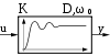
Difference equation of the delay (PT1 element)

Rectangular approximation of a PT1 element by calculation with a difference equation.

Compare picture according to Prof. Dipl.-Ing Manfred Ottens, system theory, FH-Berlin.

Transfer function of the PT1 element

${\displaystyle G(s)={\frac {Y(s)}{U(s)}}={\frac {K_{PT}}{1+s\cdot T_{1}}}={\frac {\frac {K_{PT}}{T_{1}}}{s+{\frac {1}{T_{1}}}}}}$

Associated differential equation

${\displaystyle {\dot {y}}(t)+{\frac {1}{T_{1}}}\cdot y(t)={\frac {K_{PT}}{T_{1}}}\cdot u(t)}$

The differential quotient of the differential equation is replaced by the difference quotient with the following approach:

${\displaystyle {\frac {y_{(k)}-y_{(k-1)}}{\Delta t}}+{\frac {1}{T_{1}}}\cdot y_{(k)}={\frac {K_{PT}}{T_{1}}}\cdot u_{(k)}}$

This equation is solved for y _(k) .

${\displaystyle y_{(k)}+{\frac {\Delta t}{T_{1}}}\cdot y_{(k)}=y_{(k-1)}+{\frac {K_{PT}\cdot \Delta t}{T_{1}}}\cdot u_{(k)}}$

The difference equation of the PT1 element is:

${\displaystyle y_{(k)}={\frac {T_{1}}{T_{1}+\Delta t}}\cdot y_{(k-1)}+{\frac {\Delta t\cdot K_{PT}}{T_{1}+\Delta t}}\cdot u_{(k)}}$

Difference equation of the PT1 element in simplified notation with an identical mathematical function:

${\displaystyle y_{(k)}=y_{(k-1)}+(K_{PT}\cdot u_{(k)}-y_{(k-1)})\cdot {\frac {\Delta t}{T_{1}+\Delta t}}}$

Difference equation of the proportional-differential function (ideal PD1 term)

Transfer function PD1 element:

${\displaystyle G(s)={\frac {Y(s)}{U(s)}}=K_{PD}\cdot (T_{V}\cdot s+1)}$

The corresponding differential equation is:

${\displaystyle y(t)=K_{PD}\cdot T_{V}\cdot {\dot {u}}(t)+K_{PD}\cdot u(t)}$

The differential quotient of the differential equation is replaced by the differential algorithm with the following approach:

${\displaystyle y_{(k)}=K_{PD}\cdot T_{V}\cdot {\frac {u_{(k)}-u_{(k-1)}}{\Delta t}}+K_{PD}\cdot u_{(k)}}$

The difference equation of the ideal PD1 term is:

${\displaystyle y_{(k)}=K_{PD}\cdot [u_{(k)}+(u_{(k)}-u_{(k-1)})\cdot {\frac {T_{V}}{\Delta t}}]}$

Note: Differentiating systems without so-called parasitic time constants of PT1 elements cannot be technically produced as hardware. The parasitic time constant is much smaller than the time constant of the differentiator. Nevertheless, one can numerically calculate with ideal differentiators, the size of the impulse of the step response is inversely proportional to the size of Δ t . Only when energetic provision is made as a manipulated variable in a control loop does the downstream hardware result in an unavoidable time delay.

Advantages and disadvantages of the Euler method

The calculation of difference equations according to Euler forwards or Euler backwards are practically identical in terms of accuracy.

• With the Euler reverse method, an input signal can be recorded and calculated as a pulse function (shock function) for and duration . With the Euler forward method, the input signal, the pulse function, is no longer available for the calculation of the 2nd follow-up element. All members become zero. ${\displaystyle t=0}$ ${\displaystyle h}$
• With increasing reduction of the step size and with a given input signal, the functions of both Euler methods become the same. ${\displaystyle h}$

Higher order difference equation

Example of the development of a difference equation '' 'to calculate the step response of a -link with complex conjugate poles: ${\displaystyle PT2_{kk}}$

After inserting the difference quotients instead of the differential quotients of the differential equation of a dynamic system of 1st and 2nd order, the difference equation created in this way can be solved.

Step response of a PT2 element with conjugate complex poles. Δt = 0.01 s.
${\displaystyle 0{,}25{\ddot {y}}(t)+0{,}125{\dot {y}}(t)+y(t)=1(t)}$

Given: Transfer function in the s range: ${\displaystyle G(s)={\frac {Y(s)}{U(s)}}={\frac {1}{0{,}25s^{2}+0{,}125s+1}}}$ Step function: u (t) = 1 Wanted: 2nd order difference equation for the numerical determination of the system time behavior. ${\displaystyle y_{(k)}}$ Associated differential equation according to the differentiation theorem of the Laplace transform: ${\displaystyle 0{,}25{\ddot {y}}(t)+0{,}125{\dot {y}}(t)+y(t)=u(t)}$ The difference quotients for and are inserted into the following difference equation: ${\displaystyle {\ddot {y}}(t)}$ ${\displaystyle {\dot {y}}(t)}$ ${\displaystyle 0{,}25\cdot {\frac {y_{(k)}-2y_{(k-1)}+y_{(k-2)}}{h^{2}}}+0{,}125\cdot {\frac {y_{(k)}-y_{(k-1)}}{h}}+y_{k}=u_{k}\quad |\qquad y(t)\to y_{(k)};\ u(t)\to u_{(k)}}$ The fractions are resolved into individual additive terms in order to be able to release, auxiliary variable introduced: ${\displaystyle y_{(k)}}$ ${\displaystyle \psi }$ ${\displaystyle y_{(k)}{\bigg (}{\frac {0{,}25}{h^{2}}}+{\frac {0{,}125}{h}}+1{\bigg )}:=y_{(k)}\cdot \psi =u_{(k)}+{\frac {0{,}5y_{(k-1)}}{h^{2}}}-{\frac {0{,}25y_{(k-2)}}{h^{2}}}+{\frac {0{,}125y_{(k-1)}}{h}}}$ ${\displaystyle y_{(k)}={\frac {u_{(k)}}{\psi }}+{\frac {0{,}5y_{(k-1)}}{\psi \cdot h^{2}}}-{\frac {0{,}25y_{(k-2)}}{\psi \cdot h^{2}}}+{\frac {0{,}125y_{(k-1)}}{\psi \cdot h}}\quad {\bigg |}\qquad \psi ={\frac {0{,}25}{h^{2}}}+{\frac {0{,}125}{h}}+1;\quad u_{(k)}=1}$ Calculation example for some values ​​of the output sequence with jump : ${\displaystyle y_{(k)}}$ ${\displaystyle h=0{,}01;\ \psi =2513{,}5;}$ ${\displaystyle u_{(k)}=1}$ ${\displaystyle t_{0}=0{,}00\,\mathrm {s} ;\qquad y_{(k=0)}=0{,}0004+0-0+0=0{,}0004}$. ${\displaystyle t_{1}=0{,}01\,\mathrm {s} ;\qquad y_{(k=1)}=0{,}0004+0{,}0008-0+0=0{,}0012}$. ${\displaystyle t_{2}=0{,}02\,\mathrm {s} ;\qquad y_{(k=2)}=0{,}0004+0{,}0024-0{,}0004+0=0{,}0024}$. ${\displaystyle t_{157}=1{,}57\,\mathrm {s} ;\qquad y_{(k=157)}=0{,}0004+3{,}286-1{,}643+0{,}008=1{,}652}$.

This difference equation corresponds to a recursion algorithm of a dynamic system, which can be solved step by step with a personal computer.

The recursive calculation of the 2nd order difference equation relates to the current output sequence by inserting the previous values ​​of the output sequence and into the equation. For the 1st sequential element of the calculation sequence k = 0, the previous values ​​of the initial sequence are not yet available and are therefore zero. The number of elements of the output sequence is determined by the discrete time and by the desired total time to be observed for the transient process. ${\displaystyle y_{(k)}}$ ${\displaystyle u_{(k-1)}}$ ${\displaystyle u_{(k-2)}}$ ${\displaystyle k=(0,1,2,3,\dotsc ,k_{\mathrm {max} })}$ ${\displaystyle h=\Delta t}$

Test signals

The non-periodic (deterministic) test signals are of central importance in systems theory. With their help it is possible to test a transmission system, check it for stability or determine properties.

${\displaystyle \to }$see controlled system # test signals

Accuracy of the numerical calculation using the Euler method

• The approximation error to an analytic function according to Euler forwards or Euler backwards falls linearly with decreasing step size . If , then the approximation error is about 0.1%. ${\displaystyle h}$ ${\displaystyle h=0,001}$
• The approximation error to an analytic function according to the "central Euler method" falls with the square of . ${\displaystyle h}$
• The rounding error must be taken into account if the following links are not calculated with sufficient precision. Otherwise, the rounding errors add up with every subsequent link.
• Second order difference equations as vibration terms

Second order difference equations, which describe dynamic systems in the time domain, represent a damping with complex conjugate poles as an oscillation element. Such systems contain damped sinusoidal oscillations that occur with rapid rise and fall rates. For the consideration of the accuracy of the approximation, it is decisive how many sequences take place within the first oscillation with the steepest gradient. ${\displaystyle 0<D<1}$

The greatest rate of change of a damped sinusoidal oscillation is at the 1st zero crossing and decreases with every further zero crossing.

As a rough approximation of the analytical function with the asymptote 1, the first positive half-wave should be given a resolution of more than 100 sequences . The maximum approximation error to be expected for is approx. 1%. ${\displaystyle >100\cdot \Delta t}$ ${\displaystyle y_{(k)}=f(\Delta t=0{,}003)}$

The number of episodes for a period of time has no influence on the accuracy. ${\displaystyle k_{\mathrm {max} }\cdot \Delta t}$

Non-linear transmission systems

Relatively simple transmission system structures with non-linear elements can no longer be solved in a closed manner by conventional calculation methods in the continuous time domain.

General representation of a non-linear transmission link based on the Hammerstein model

According to the Hammerstein model, the non-linear system behavior is considered in a static non-linear model in connection with a series connection with a linear dynamic system.

Measures for the linearization of non-linear transmission systems:

• Limitation effects : simulation of the limitation with logical instructions,
• Non-linear characteristic: the use of a model control loop forces linearity,
• Non-linearity: through logical commands such as logical instructions e.g. B. IF-THEN-ELSE statements or tables that describe the static non-linearity.
• System dead : calculating an approximation model with delays or higher order all-pass filter, ${\displaystyle Tt}$

Storage of subsequent members with access to chronologically past members. ${\displaystyle Tt}$

• Hysteresis: The non-linear function is stored in tables.

${\displaystyle \to }$See also picture control engineering # non-linear transmission system

${\displaystyle \to }$See also dead time (control technology) # Approach to the behavior of a dead time element through PTn elements as a substitute dead time

z-transfer function

If the right shift theorem of the z-transformation is applied to difference equations, the z-transfer function of the discrete system is obtained directly as the ratio of the z-transforms of the input and output sequence. The following information about the application with linear systems:

• The difference equations can only be transferred into the complex z-image area and into the z-transfer functions with the aid of the linearity theorem and the displacement theorem . ${\displaystyle y_{(k)}}$ ${\displaystyle G(z)=Y(z)/U(z)}$
• Given transfer functions of the s-area in connection with holding elements and sensing elements can also be transformed as z-transfer functions with the help of the z-correspondence tables.
• The z-transfer function is:

${\displaystyle G(z)={\frac {Y(z)}{U(z)}}={\frac {{\text{Zählerpolynom}}\ (z)}{{\text{Nennerpolynom}}\ (z)}}}$.

• The inverse transformation from the z-transfer function into the discrete-time domain as a difference equation is carried out by the inversely applied linearity law and shift law for all individual terms.

Application of the z-transfer function in a control loop

See also z-transformation # Application of the z-transfer function for a digital PI controller with sampling function and holding element .

Both sampled input signals u (kT _A ) and difference equations f (kT _A ), which describe the behavior of a system in the discrete time domain (e.g. the control algorithm of a controller), can be transformed into the z domain as z transfer functions and treated as algebraic equations.

If an inverse z-transformation of the z-transfer functions is carried out, the solution of the time-discrete difference equation arises in the range. With the help of various methods of reverse transformation from the z-domain to the time-discrete k-domain, the solution is then obtained as the difference equations of the control algorithm for the discrete domain f (kT _A ). ${\displaystyle f_{(k)}={\mathcal {Z}}^{-1}\{F(z)\}}$ ${\displaystyle f(kT_{A})}$

The typical application procedure of the z-transformation on a digital system, a digital controller or a digital filter is as follows for the control algorithm:

• The sampling sequence of the input signal (input sequence) is transformed as a z-transfer function , ${\displaystyle H(z)}$
• The difference equation of the desired controller behavior is transformed as a z-transfer function , ${\displaystyle f_{(k\cdot T_{A})}}$ ${\displaystyle G(z)}$
• The z-transformed systems are grouped algebraically according to the z-calculation rules,
• With the inverse z-transformation of the z-product of the signal and the control algorithm, the calculation algorithm of the digital controller (microcomputer) is again created as a difference equation.

The analysis and synthesis of discrete signals and systems can be facilitated with the z-transformation, but also requires extensive mathematical special knowledge that is partly based on rules similar to those of the Laplace transformation.

${\displaystyle \to }$See article z-transformation .

Difference Equations in Economics

In economic theory, difference equations are mainly used to analyze the development of economic variables over time. In growth theory and business cycle theory in particular , temporal processes are often mapped in the form of difference equations.

It is assumed that z. B. the gross domestic product develops on a certain path towards a long-term equilibrium in which all capacities are fully utilized. Depending on the solution of the difference equation, the development path results as an asymptotic course or as an oscillating course (roughly cosine curves). However, it is inevitable that some simplifying assumptions have to be made for mathematical modeling (e.g. for gross domestic product) (e.g. about inventory formation, consumption as a share of GDP or investment increase through profit expectations).

• Application of first order difference equation

Another classic example is the cobweb model (also cobweb theorem ). The development of prices and quantities follows recursive functions or, in mathematical terms, general first-order difference equations.

• Application of the second order difference equation

The multiplier-accelerator model aims to explain why economic growth is not monotonous, but typically follows an economic cycle. The model can be developed from the growth model of Harrod and Domar , a special variant comes from Paul A. Samuelson (1939) and John Richard Hicks (1950).

See also

• Generating function
• Difference calculation
• Numerical Recipes Programs for solving differential equations in common programming languages

literature

• May-Britt Kallenrode: Computational Methods in Physics: Mathematical Companion to Experimental Physics , Springer, 2005
• Paul Cull, Mary Flahive, Robby Robson: Difference equations. From Rabbits to Chaos , Springer, Undergraduate Texts in Mathematics, 2005
• Holger Lutz, Wolfgang Wendt: Pocket book of control engineering with MATLAB and Simulink . 11th edition. Europa-Lehrmittel, 2019, ISBN 978-3-8085-5869-0 .
• Gerd Schulz: Control technology 2 / multi-variable control, digital control technology, fuzzy control . 2nd Edition. Oldenbourg, 2008, ISBN 978-3-486-58318-2 .
• Jan Lunze: Control engineering 2, multi-variable systems, digital control . 7th edition. Springer Verlag, 2013, ISBN 978-3-642-10197-7 .
• Krause, Nesemann: difference equations and discrete dynamic systems. An introduction to theory and applications. 1999th edition. Vieweg + Teubner Verlag, 1999, ISBN 978-3-519-02639-6 .
• Alan V. Oppenheim, RW Schafer: Discrete-time signal processing . Pearson Education, Upper Saddle River, NJ 2004, ISBN 3-8273-7077-9 .

Web links

Wikibooks: Linear recurrences, power series and their generating functions  - learning and teaching materials

• 13. Difference equations. Chapter on difference equations with mathematical examples, University of Greifswald (PDF; 52 kB).

Individual evidence

1. ↑ Jürgen Koch, Martin Stämpfle: Mathematics for engineering studies . Hanser, 2015, ISBN 978-3-446-44454-6 , pp. 545–546 ( limited preview in Google Book search).
2. ↑ Barbara Wohlmuth: Numerical Methods for Ordinary Differential Equations. (PDF) In: Script, TU Munich, Chair for Numerical Mathematics. Retrieved July 16, 2020 . 
3. ↑ Jürgen Dankert: Numerical integration of initial value problems. Script, HAW-Hamburg, 39 pages.
4. ^ Lutz, Wendt: Pocket book of control engineering. Chapter Basic Algorithms for Digital Controls.
5. ↑ ^{a b} Herbert Oertel jr., Martin Böhle, Thomas Reviol: Fluid mechanics: Fundamentals - basic equations - solution methods ... 6th edition. Vieweg + Teubner, 2011, ISBN 978-3-8348-1397-8 , pp. 364 ( limited preview in Google Book search).
6. ↑ Prof. Dr. Johannes Wandinger, University of Munich, script "Numerical Methods, Initial Value Problem". Call up from Google: Euler forward, then 1st order initial value problem, Prof. Dr. Wandinger
7. ↑ Treatise Taylor series development: tu-berlin.de/Lehre/tfd_skript/node11.html
8. ↑ Script “Fundamentals of System Theory”, Prof. Dipl.-Ing. Manfred Ottens, FH Berlin, see “Continuous and time-discrete signals and systems” and “Output sequence of the time-discrete delay element”.
9. ↑ difference equation. Definition in the Gabler Wirtschaftslexikon.
10. ↑ Arthur Woll: General Economics. Vahlen Franz GmbH, 12th edition, 1996, ISBN 3800629739 , page 111 for the mathematical derivation.
11. ↑ Multiplier-accelerator models. Definition in the Gabler Wirtschaftslexikon.