SI model

In mathematical epidemiology , a branch of theoretical biology , the SI model represents a particularly simple approach to describing the spread of contagious diseases, whereby all healthy people are ultimately infected.

Model description

Designate at the time ${\textstyle t}$

${\displaystyle S(t)}$  the healthy, not yet infected individuals ( susceptible individuals S)

${\displaystyle I(t)}$  the sick, already infected individuals ( infectious individuals I),

and for the sake of simplicity let us assume d. H. the considered population consists of individuals at all times (which means that births and deaths are not taken into account). I.e. the increase in infected individuals in the unit of time corresponds to the decrease in healthy individuals in the unit of time. ${\textstyle I(t)+S(t)=N=\mathrm {const} }$ ${\textstyle t}$ ${\textstyle N}$

The rate of spread of the disease is statistically dependent on the one hand on the number of sick individuals (i.e. the number of germ carriers) and on the other hand on the number of individuals who can still be infected.

The simplest approach uses a linear functional response like the law of mass action with an interaction term : ${\textstyle c}$

${\displaystyle {\frac {\mathrm {d} S}{\mathrm {d} t}}=-c\cdot I(t)\cdot S(t)}$,

${\displaystyle {\frac {\mathrm {d} I}{\mathrm {d} t}}=c\cdot I(t)\cdot S(t)}$.

The product can be interpreted as the number of contacts when all healthy people interact with all infected people, and the factor determines the resulting new infections (infection rate). Taking advantage of the above conservation law , from which it follows, we can write ${\textstyle I(t)\cdot S(t)}$ ${\textstyle c}$ ${\textstyle S(t)=N-I(t)}$

${\displaystyle {\frac {\mathrm {d} I}{\mathrm {d} t}}=c\cdot I(t)\left(N-I(t)\right)=c\cdot N\cdot I(t)\left(1-{\frac {I(t)}{N}}\right)}$.

The proportionality factor cN is determined from the initial exponential growth . For this purpose I (t) << N applies and the above differential equation changes into

${\displaystyle {\frac {\mathrm {d} I}{\mathrm {d} t}}=c\cdot N\cdot I(t)=r\cdot I(t)}$

with r as the replication rate (reciprocal half-life ) independent of the total population N. From this it follows:

${\displaystyle {\frac {\mathrm {d} I}{\mathrm {d} t}}=r\cdot I\cdot (1-{\frac {I}{N}})}$.

The two determining differential equations are written as follows:

${\displaystyle {\frac {\mathrm {d} S}{\mathrm {d} t}}=-\left[r\cdot S(t)\right]\cdot I(t)}$,

${\displaystyle {\frac {\mathrm {d} I}{\mathrm {d} t}}=\left[r\cdot I(t)\right]\cdot S(t)}$

results in the comparison with the predator-prey behavior (infected-healthy!). However, this does not lead to a vibration equation as in the predator-prey behavior.

Extensions of the SI model are the SIS model , in which healthy individuals can, and the SIR model , in which individuals immune to the disease can be.

Analytical solution of the differential equation of the SI model

Course of the number of infected I and healthy S

1. Derivation of the infected I as a function of time t

1st and 2nd derivative of the infected I as a function of I

According to the integral table, the solution to this differential equation is

${\displaystyle I(t)={\frac {N}{1+\left({\frac {N}{I(0)}}-1\right)\cdot e^{-rt}}}={\frac {N}{1+e^{-r\left(t-tw\right)}}}}$

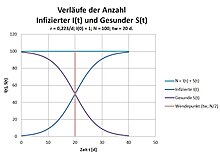
with time for the turning point of I (t)

${\displaystyle tw={\frac {ln\left({\frac {N}{I\left(0\right)}}-1\right)}{r}}}$.

According to the conservation law we get for the complementary variable S:

${\displaystyle {\frac {\mathrm {d} S}{\mathrm {d} t}}=-r\cdot S\cdot (1-{\frac {S}{N}})}$ and

${\displaystyle S(t)={\frac {N\cdot e^{-r\left(t-tw\right)}}{1+e^{-r\left(t-tw\right)}}}={\frac {N}{1+e^{r\left(t-tw\right)}}}}$.

It applies

${\displaystyle I(\infty )=N}$,

${\displaystyle {\frac {dI}{dt}}={\frac {r\cdot N\cdot ({\frac {N}{I(0)}}-1)\cdot e^{-rt}}{[1+({\frac {N}{I(0)}}-1)\cdot e^{-rt}]^{2}}}}$.

In words: all healthy people are infected.

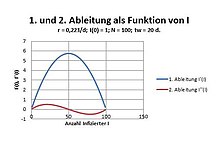
The first time derivative of I (t) is an equation of the second degree with respect to N with zeros 0 and N. The maximum occurs at the inflection point of I (t)

${\displaystyle {\frac {\mathrm {d} I}{\mathrm {d} t}}|tw={\frac {r\cdot N}{4}}}$.

The second time derivative of I (t) is also of interest:

${\displaystyle {\frac {\mathrm {d} ^{2}I}{\mathrm {d} t^{2}}}=r^{2}\cdot N\cdot (1-{\frac {2I}{N}})\cdot (1-{\frac {I}{N}})}$

It has three zeros at 0, N / 2 and N. Between the first two zeros there is a maximum:

${\displaystyle I_{1}={\frac {N}{2}}\cdot (1-{\frac {1}{\sqrt {3}}})=0,2213\cdot N}$

${\displaystyle {\frac {d^{2}I}{dt^{2}}}|I_{1}={\frac {r^{2}\cdot N}{6\cdot {\sqrt {3}}}}=0,09623\cdot r^{2}\cdot N}$,

a minimum between the last two zeros:

${\displaystyle I_{2}={\frac {N}{2}}\cdot (1+{\frac {1}{\sqrt {3}}})=0,77887\cdot N}$

${\displaystyle {\frac {d^{2}I}{dt^{2}}}|I_{2}=-{\frac {d^{2}I}{dt^{2}}}|N_{1}=-0,09623\cdot r^{2}\cdot N.}$

The relative time change of I (t), called Q, is suitable for determining r and N of a real distribution:

${\displaystyle Q(t)={\frac {\frac {\mathrm {d} I}{\mathrm {d} t}}{I}}=r\cdot \left(1-{\frac {I}{N}}\right)}$.

Q (I) decreases linearly with increasing I. It applies

${\displaystyle Q(I=0)=r}$,

${\displaystyle Q(I=N)=0}$.

Using regression analysis e.g. In this way, e.g. using Excel, r and N can be determined quickly and easily for a real distribution.

Reproduction rate of the Robert Koch Institute in the SI model

Reproduction rate of the Robert Koch Institute in the SI model

For distributions of this kind, a reproduction rate according to the Robert Koch Institute R _RKI, also called R value, has become important in the COVID-19 pandemic :

${\displaystyle R_{\text{RKI}}(t)={\frac {I(t)-I(t-s)}{I(t-s)-I(t-2s)}}}$ with s = 4 and t ≥ 2s.

If I (t) is replaced by the solution function, the result is

${\displaystyle R_{\text{RKI}}(t)=e^{-rs}\cdot {\frac {1+({\frac {N}{I(0)}}-1)e^{-r\left(t-2s\right)}}{1+({\frac {N}{I(0)}}-1)e^{-rt}}}}$

With

${\displaystyle R_{\text{RKI}}(-\infty )=e^{rs}}$,

${\displaystyle R_{\text{RKI}}(2s)=e^{-rs}\cdot {\frac {1+({\frac {N}{I(0)}}-1)}{1+({\frac {N}{I(0)}}-1)\cdot e^{-2rs}}}\thickapprox e^{rs}}$,

${\displaystyle R_{\text{RKI}}(\infty )=e^{-rs}}$ .

The R-value has the following additional properties:

${\displaystyle R_{\text{RKI}}(tw)={\frac {e^{rs}+e^{-rs}}{2}}}$,

${\displaystyle R_{\text{RKI}}(tw+s)=1}$,

${\displaystyle R_{\text{RKI}}(I)=e^{rs}-{\frac {e^{rs}-e^{-rs}}{N}}\cdot I}$.

The R-value consequently decreases linearly with increasing numbers of infections.

Behavior with r-drop and 2nd wave

Course of the infected persons over time: without r decrease according to the SI model: I1, after r decrease at 10 d according to the SI model: I2 and after an r jump with a linear course: I3

1. Temporal guidance of the infected over time: without r-decrease according to the SI model: I'1 and after r-decrease at 10 d according to the SI model: I'2

R value (= RRKI) over time: without r decrease according to SI model: RRKI1 and after r decrease at 10 days according to SI model: RRKI2

The approach

${\displaystyle {\frac {dI}{dt}}=r\cdot I\cdot (1-{\frac {I}{N}})}$

can be written

${\displaystyle {\frac {dI}{dt}}=r_{\text{eff}}\cdot I{\text{ mit }}r_{\text{eff}}=(1-{\frac {I}{N}}).}$

While the replication rate r is defined independently of time in the SI model, here reff is indirectly time-dependent via I (t) and decreases with increasing time, which results in a parabolic curve that is open at the bottom for the first time derivative of the infected I (t). Instead of an indirect time dependency, a direct time dependency is now used. In the pictures of the selected example, r is suddenly reduced at ts = 10 d to r2 = r / 7 before the turning point at tw = 20 d. The calculation is carried out with the difference equation in daily steps instead of the differential equation numerically using Excel, which results in slight differences that, however, have no influence on the basic behavior. At I (t) there is a kink to a flatter curve in accordance with the lower replication rate and at dI / dt a maximum similar to that of the aforementioned example. The flattening of I (t) leads to a new turning point

${\displaystyle t_{\text{ws}}\approx t_{s}<t_{w},}$

thereby simulating a smaller total amount N of the population. Concrete examples of this are the infection curves of various countries for CORVID-19. Furthermore, variables and parameters of the primary infection are given the index 1 to differentiate, those after the r decrease with the index 2. The point I1 (tws) is the starting value of a new infection curve

${\displaystyle I_{2}(0)=I_{2}(t-t_{s})=I_{1}(t_{\text{ws}})}$

with the turning point at

${\displaystyle t_{\text{w2}}=ln{\frac {N}{I_{2}(0)-1}}+t_{s}}$

and a maximum of change from

${\displaystyle {\frac {dI_{2}}{dt}}|max={\frac {r_{2}\cdot N}{4}}<{\frac {r_{1}\cdot N}{4}}.}$

However, 100 percent infection does not yet occur after the r decrease, but this does not occur until later according to the I2 development and, based on the aforementioned assumptions, corresponds to the second wave.

Termination of the exponential infected behavior and conclusion

If the second wave is predicted after a drop in r, the question arises of how to prevent it. How can this behavior be prevented or at least reduced? The SI model states that if the replication rate r is positive and not zero, all healthy individuals are infected. It is only a matter of when! A termination only takes place with r = 0. The realization of this is z. B. not possible with CORVID-19 in 2020. It would be an absolute lockdown ! A (renewed) exponential increase in time of dI / dt can only be prevented by forcing a polynomial increase in time, in the simplest case a linear increase in time as follows:

${\displaystyle {\frac {dI_{3}}{dt}}=k=const}$with . ${\displaystyle {\frac {d^{2}I_{3}}{dt^{2}}}=0}$

This approach continues to apply

${\displaystyle I_{3}(t)=k\cdot t+I_{\text{30}}}$ and ${\displaystyle R_{RKI}=1.}$

For the period before the 2nd turn tw2 applies

${\displaystyle {\frac {d^{2}I_{2}}{dt2}}>0}$ and consequently ${\displaystyle {\frac {d^{2}I_{2}}{dt^{2}}}>{\frac {d^{2}I_{3}}{dt^{2}}}.}$

In words: the linear growth always remains below the exponential growth. As soon as the forced state is exited, the SI model becomes effective with the 2nd wave. In this way, the yes or no of a second wave can be distinguished. This linear behavior corresponds to an unstable equilibrium . In real terms, this means that the exponentially developing chains of infection should be interrupted as far as possible at their origin, as with CORVID-19 z. B. for Germany in the period from May to July 2020. As soon as the compulsion is removed, the avalanche of exponential development begins again! On the other hand, the compulsion causes a sensible delay until the growth of the infected person ceases to exist, e.g. through immunization, etc.

See also

• SIS model (spread of infectious diseases without building up immunity)
• SIR model (spread of infectious diseases with immunity formation)
• SEIR model (spread of contagious diseases with immunity development, in which infected people are not immediately infectious)
• Base reproduction number
• Dynamic system (mathematical generic term)

literature

• James D. Murray : Mathematical Biology . Springer, 1993, ISBN 3-540-57204-X .

Individual evidence

1. ↑ Integral table. Accessed July 12, 2020 (Formula 17 on page 1). 
2. ↑ COVID-19 pandemic in Germany # reproduction number
3. ↑ basic reproduction number # calculation of the basic reproduction number

Remarks

1. ↑ An abstract example: An infected person infects two other people in one day, i.e. a total of 3, the two newly infected people each infect two, i.e. four, i.e. a total of 7 etc. In mathematical terms, this means: 2 ^t -1 or e ^rt -1 with r = ln2 = 0.693. A real example: exponential initial growth of the infected with Corona: Germany with 83 million inhabitants: r = 0.315 / d; Saxony with 4.2 million inhabitants: r = 0.354 / d; Austria with 8.9 million inhabitants: r = 0.324 / d, regardless of the number of inhabitants.