Silhouette coefficient

The silhouette indicates an observation of how good is the assignment to the two nearest clusters. The silhouette coefficient indicates a measure of the quality of a clustering that is independent of the number of clusters . The silhouette plot visualizes all the silhouettes of a data set as well as the silhouette coefficient for the individual clusters and the entire data set.

silhouette

structuring	Range of values from ${\ displaystyle S (o)}$
strong	${\ displaystyle 0 {,} 75 <S (o) \ leq 1}$
medium	${\ displaystyle 0 {,} 5 <S (o) \ leq 0 {,} 75}$
weak	${\ displaystyle 0 {,} 25 <S (o) \ leq 0 {,} 5}$
no structure	${\ displaystyle 0 <S (o) \ leq 0 {,} 25}$

If the object belongs to the cluster , the silhouette of is defined as: ${\ displaystyle o}$ ${\ displaystyle A}$ ${\ displaystyle o}$

{\ displaystyle S (o) = {\ begin {cases} 0 & {\ text {if}} o {\ text {only element of}} A {\ text {is}} \\ {\ frac {\ operatorname {dist } (B, o) - \ operatorname {dist} (A, o)} {\ max \ {\ operatorname {dist} (A, o), \, \ operatorname {dist} (B, o) \}}} & {\ text {otherwise}} \ end {cases}}}

with the distance of an object to the cluster and the distance of an object to the closest cluster . The difference in the distance is normalized with the maximum distance. It follows that for an object lies between −1 and 1: ${\ displaystyle \ operatorname {dist} (A, o)}$ ${\ displaystyle o}$ ${\ displaystyle A}$ ${\ displaystyle \ operatorname {dist} (B, o)}$ ${\ displaystyle o}$ ${\ displaystyle B}$ ${\ displaystyle \ operatorname {dist} (B, o) - \ operatorname {dist} (A, o)}$ ${\ displaystyle S (o)}$ ${\ displaystyle o}$

If the silhouette is , then the objects in the closest cluster are closer to the object than the objects in the cluster to which the object belongs. This indicates that clustering can be improved. ${\ displaystyle S (o) <0}$ ${\ displaystyle B}$ ${\ displaystyle o}$ ${\ displaystyle A}$ ${\ displaystyle o}$
If the silhouette , then the object lies between two clusters and ${\ displaystyle S (o) \ approx 0}$
if the silhouette is close to one, the object is in a cluster.

The distance is calculated as ${\ displaystyle \ operatorname {dist} (A, o)}$

{\ displaystyle \ operatorname {dist} (A, o) = {\ frac {1} {n_ {A} -1}} \ sum _ {a \ in A, a \ neq o} \ operatorname {dist} (a ,O)}

as the mean of the distance between all other objects in the cluster and the object ( is the number of objects in the cluster ). Similarly, the distance to the closest cluster is calculated as the minimum average distance ${\ displaystyle A}$ ${\ displaystyle o}$ ${\ displaystyle n_ {A}}$ ${\ displaystyle A}$ ${\ displaystyle B}$

{\ displaystyle \ operatorname {dist} (B, o) = \ min _ {C \ neq A} \ underbrace {\ left ({\ frac {1} {n_ {C}}} \ sum _ {c \ in C } \ operatorname {dist} (c, o) \ right)} _ {= \ operatorname {dist} (C, o)}}

.

The distance is calculated for all clusters that do not contain the object . The closest cluster is the one that is closest . ${\ displaystyle C}$ ${\ displaystyle o}$ ${\ displaystyle \ operatorname {dist} (C, o)}$ ${\ displaystyle B}$ ${\ displaystyle \ operatorname {dist} (C, o)}$

Silhouette coefficient

The silhouette coefficient is defined as ${\ displaystyle s_ {C}}$

{\ displaystyle s_ {C} = {\ tfrac {1} {n_ {C}}} \ sum _ {o \ in C} s (o)}

thus defined as the arithmetic mean of all the silhouettes in the cluster . The silhouette coefficient can be calculated for each cluster or for the entire data set. ${\ displaystyle n_ {C}}$ ${\ displaystyle C}$

With the k-means or k-medoid algorithm, it can be used to compare the results of several runs of the algorithm in order to obtain better parameters. This is particularly useful for the algorithms mentioned, since they start randomly and can thus find different local maxima. The influence of the parameter can thus be reduced, since the silhouette coefficient is independent of the number of clusters and can thus compare results that were obtained with different values for . ${\ displaystyle k}$ ${\ displaystyle k}$

Silhouette plot

The graphical representation of the silhouettes takes place for all observations together in a silhouette plot . For all observations that belong to a cluster, the value of the silhouette is shown as a horizontal (or vertical) line. The observations in a cluster are arranged according to the size of the silhouettes.

The graph on the right shows the data for four different data sets, the dendrogram for a hierarchical cluster analysis (Euclidean distance, single linkage) and the silhouette plot for the solution with two clusters (from top to bottom). The assignment of the data points by the hierarchical cluster analysis in the two-cluster solution is symbolized by the colors red (assignment to cluster 1) and blue (assignment to cluster 2).

The better the two clusters are separated in the data (from left to right), the better the hierarchical cluster analysis can assign the data points correctly. The silhouette plot also changes. While negative silhouettes occur for the data set on the left, only positive silhouettes are found in the data set on the far right. The silhouette coefficients also increase from left to right, both for the individual clusters and for the entire data set.

example

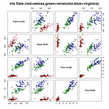
The Iris flower dataset consists of 50 observations of three species of irises (Iris Setosa, Iris Virginica and Iris Versicolor), on each of which four attributes of the flowers were recorded: the length and width of the sepalum (sepal) and the petalum (petal ). On the right, a scatter plot matrix shows the data for the four variables.

Dendrogram and silhouette plot for a two-, three-, and four-cluster solution.

A hierarchical cluster analysis with the Euclidean distance and the single linkage method was carried out for the four quantities . The following graphics are shown above:

Top left : A dendrogram of the cluster solution. Here you can see that a two- or four-cluster solution would be appropriate.
Top right : Graphical representation of the silhouettes of the two-cluster solution. Negative silhouettes can be found in the first cluster so that these observations are more likely to be assigned incorrectly. A solution with more clusters may be more suitable. ${\ displaystyle S (o)}$
Bottom left : Graphic representation of the silhouettes of the three-cluster solution. The first cluster is split into two sub-clusters ( ); Although the negative silhouettes in the first cluster have disappeared, observations in the second cluster now have negative silhouettes. ${\ displaystyle 78 = 50 + 28}$
Bottom right : Graphic representation of the silhouettes of the four-cluster solution. The second cluster of the two-cluster solution is now split into two sub-clusters ( ). There are almost no negative silhouettes left. ${\ displaystyle 72 = 60 + 12}$

The following silhouette coefficients result

	Silhouette coefficients ${\ displaystyle n_ {C} / s_ {C}}$
Number of clusters	Total
2	150 / 0.52	78 / 0.39		72 / 0.66
3	150 / 0.51	50 / 0.76	28 / 0.59	72 / 0.31
4th	150 / 0.50	50 / 0.76	28 / 0.52	60 / 0.27	12 / 0.51

literature

Martin Ester, Jörg Sander: Knowledge Discovery in Databases: Techniques and Applications . Springer, Hamburg / Berlin 2000, ISBN 3-540-67328-8 , pp. 66 . Online: limited preview in Google Book search
Peter J. Rousseeuw: Silhouettes: a Graphical Aid to the Interpretation and Validation of Cluster Analysis . In: Computational and Applied Mathematics. 20, 1987, pp. 53-65. doi : 10.1016 / 0377-0427 (87) 90125-7 .

Web links

silhouette of: calculating coefficients and silhouette -plots with R .

Individual evidence

↑ Peter J. Rousseeuw: Silhouettes: A graphical aid to the interpretation and validation of cluster analysis . In: Journal of Computational and Applied Mathematics . No. 20 , 1987, pp. 53-65 ( online ).

[1] Peter J. Rousseeuw: Silhouettes: A graphical aid to the interpretation and validation of cluster analysis . In: Journal of Computational and Applied Mathematics . No. 20 , 1987, pp. 53-65 ( online ).