Hierarchical cluster analysis

This article covers hierarchical cluster analysis in statistics ; for other cluster analysis methods see cluster analysis .

A specific family of distance-based methods for cluster analysis (structure discovery in databases) is called hierarchical cluster analysis . In this case, clusters consist of objects that are closer to one another (or, conversely, are more similar) than to objects in other clusters. The methods in this family can be differentiated according to the distance or proximity measures used (between objects, but also between entire clusters) and according to their calculation rules.

If one subdivides according to the calculation rule, one differentiates between two important types of procedures:

• the divisive cluster method, in which all objects are initially considered to belong to a cluster and then the already formed clusters are gradually divided into smaller and smaller clusters until each cluster consists of only one object. (Also referred to as the " top-down procedure ")
• the agglomerative clustering process, in which each object first forms a cluster and then the clusters that have already been formed are gradually combined to form larger and larger ones until all objects belong to one cluster. (Also referred to as the " bottom-up process ")

It applies to both methods that once clusters have been formed , they can no longer be changed. The structure is either only refined (“divisive”) or only coarsened (“agglomerative”) so that a strict cluster hierarchy is created. You can no longer tell from the resulting hierarchy how it was calculated.

advantages and disadvantages

The advantages of the hierarchical cluster analysis are the flexibility through the use of complex distance measures, that the method has no parameters of its own apart from the distance function and the merging method and that the result is a cluster hierarchy that also allows sub-structures.

The disadvantage is the effort required to analyze the result. Other methods, such as B. the k-means algorithm , DBSCAN or the hierarchical OPTICS algorithm, provide a single partitioning of the data in clusters. A hierarchical cluster analysis provides numerous such partitions, and the user has to decide how to partition. However, this can also be an advantage, since the user is given a summary of the qualitative behavior of the clustering. This knowledge is fundamental to topological data analysis in general, and persistent homology in particular.

Another disadvantage of hierarchical cluster analysis is the runtime complexity. An agglomerative calculation occurs much more frequently in practice and research, as there are possibilities in every step to combine clusters, which leads to a naive overall complexity of . In special cases, however, methods are known with an overall complexity of . Divisively, however, there are naively ways of dividing the data set in each step . ${\displaystyle O(n^{2})}$ ${\displaystyle O(n^{3})}$ ${\displaystyle O(n^{2})}$ ${\displaystyle O(2^{n})}$

Another disadvantage of hierarchical cluster analysis is that it does not provide any cluster models. For example, depending on the dimensions used, chain effects ("single-link effects") are created and outliers are often used to create tiny clusters that only consist of a few elements. The clusters found therefore usually have to be analyzed afterwards in order to obtain models.

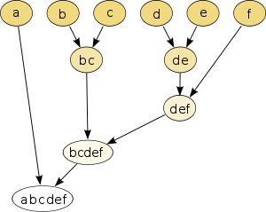
Dendrogram

• Record and dendrogram
• 

  Record. The objects and as well as and are very close together. ${\displaystyle b}$ ${\displaystyle c}$ ${\displaystyle d}$ ${\displaystyle e}$

• 

  Dendrogram for single linkage. and as well as and are summarized first. ${\displaystyle b}$ ${\displaystyle c}$ ${\displaystyle d}$ ${\displaystyle e}$

To visualize the resulting from a hierarchical clustering tree can dendrogram ( Greek. Δένδρον (dendron) = tree) are used. The dendrogram is a tree that shows the hierarchical breakdown of the amount of data into ever smaller subsets . The root represents a single cluster that contains the entire set . The leaves of the tree represent clusters, each with a single object of the data set. An inner node represents the union of all of its child nodes. Every edge between a node and one of its child nodes still has the distance between the two representing sets of objects as an attribute. ${\displaystyle O}$ ${\displaystyle O}$

Dendrogram

The dendrogram becomes more informative when an axis is used to represent the distance or (dis) similarity. If two clusters are joined together, then these clusters have a certain distance or (dis) similarity to one another. The connecting line is drawn at this height. In the example opposite, z. B. the objects RR1 and RR4 combined with a value of the similarity measure of approx. The "height" is the horizontal axis here.

In this representation, one can select a desired number of clusters by cutting through the dendrogram at an appropriate height. Typically, you are looking for a place where there is a large jump in distance or (dis) similarity between two mergers, e.g. B. in the right dendrogram at level 40. Then there are four clusters, two of which contain only individual objects (RR2, RR5), one cluster contains two objects (RR3 and RR6) and the last cluster contains all other objects. If there are hierarchical clusters with significantly different sizes, it may be necessary to split them at different levels: while one cluster is still connected to its neighbors at one level, another ("thinner") cluster already breaks down into individual objects at this level .

Distance and similarity measures

In agglomerative as well as divisive hierarchical cluster analyzes, it is necessary to calculate distances or (in) similarities between two objects, an object and a cluster or two clusters. Depending on the scale level of the underlying variables, different measures are used:

• For categorical ( nominal and ordinal ) variables, similarity measures are used; H. a value of zero means that the objects have maximum dissimilarity. These can be converted into distance measurements.
• Distance measures are used for scale variables; H. a value of zero means that the objects have a distance of zero, i.e. maximum similarity.

→ Main article : Similarity analysis

The following table shows some similarity or distance measures for binary and scale variables. Categorical variables with more than two categories can be converted into multiple binary variables. The Gower distance can also be defined for nominally scaled variables.

Similarity measure	${\displaystyle s(i,j)}$	Distance measure	${\displaystyle d(i,j)}$
Jaccard	${\displaystyle {\frac {n_{11}}{n_{01}+n_{10}+n_{11}}}}$	${\displaystyle L_{r}}$	${\displaystyle \left(\sum _{k=1}^{p}(x_{ik}-x_{jk})^{r}\right)^{1/r}}$
Tanimoto	${\displaystyle {\frac {n_{00}+n_{11}}{n_{00}+2(n_{01}+n_{10})+n_{11}}}}$	Euclidean ${\displaystyle L_{2}}$	${\displaystyle {\sqrt {\sum _{k=1}^{p}(x_{ik}-x_{jk})^{2}}}}$
Simple matching	${\displaystyle {\frac {n_{00}+n_{11}}{p}}}$	Pearson	${\displaystyle {\sqrt {\sum _{k=1}^{p}{\frac {(x_{ik}-x_{jk})^{2}}{s_{k}^{2}}}}}}$ with the standard deviation of the variable ${\displaystyle s_{k}}$ ${\displaystyle k}$
Russel Rao	${\displaystyle {\frac {n_{11}}{p}}}$	City block Manhattan ${\displaystyle L_{1}}$	${\displaystyle \sum _{k=1}^{p}|x_{ik}-x_{jk}|}$
Dice	${\displaystyle {\frac {2n_{11}}{n_{01}+n_{10}+2n_{11}}}}$	Gower	${\displaystyle \sum _{k=1}^{p}{\frac {|x_{ik}-x_{jk}|}{r_{k}}}}$ with the range of the variable ${\displaystyle r_{k}}$ ${\displaystyle k}$
Kulczynski	${\displaystyle {\frac {n_{11}}{n_{01}+n_{10}}}}$	Mahalanobis	${\displaystyle {\sqrt {(x_{i}-x_{j})^{T}S^{-1}(x_{i}-x_{j})}}}$ with the covariance matrix of the variables ${\displaystyle S}$ ${\displaystyle x_{i}}$

Examples

• An Internet bookseller knows for two visitors which book websites they have viewed , so a 0 = not viewed or 1 = viewed is stored for each of the websites . What degree of similarity is available to find out how similar the two visitors are? The number of book web pages that neither visitor viewed ( ), of which there are many, should not be included in the calculation. One possible coefficient would be the Jaccard coefficient, i. H. the number of book websites that both visitors viewed ( ) divided by the number of book websites that at least one of the two visitors viewed ( number of book websites that only the first visitor viewed, and number of book web pages that only the second visitor viewed). ${\displaystyle p}$ ${\displaystyle =n_{00}}$ ${\displaystyle =n_{11}}$ ${\displaystyle n_{10}}$ ${\displaystyle n_{01}}$
• In the ALLBUS data is u. a. Asked about the assessment of the current economic situation with the possible answers very good , good , partially , bad and very bad . A binary variable is now formed for each of the possible answers so that the binary similarity measures can be used. It should be noted that if there are several variables with different number of categories, the number of categories should be weighted .
• In the Iris dataset , the four ( ) dimensions of iris petals are considered. To calculate distances between two petals and , z. B. the Euclidean distance can be used. ${\displaystyle =p}$ ${\displaystyle i}$ ${\displaystyle j}$

Which similarity or distance measure is used ultimately depends on the desired interpretation of the content of the similarity or distance measure.

Agglomerative calculation

The agglomerative calculation of a hierarchical cluster analysis is the simplest and most flexible case. At the beginning, each object is seen as a separate cluster. Now in each step the next clusters are combined into one cluster. If a cluster consists of several objects, it must be specified how the distance between clusters is calculated. The individual agglomerative processes differ here. The method can be ended when all clusters exceed / fall below a certain distance / similarity to one another or when a sufficiently small number of clusters has been determined. This is trivial in the case of clusters with only one object, as specified at the beginning.

In order to carry out an agglomerative cluster analysis,

• a distance or similarity measure to determine the distance between two objects and
• a merging algorithm can be selected to determine the distance between two clusters.

The choice of the merging algorithm is often more important than that of the distance or similarity measure.

Merging algorithms

This article or the following section is not adequately provided with supporting documents ( e.g. individual evidence ). Information without sufficient evidence could be removed soon. Please help Wikipedia by researching the information and including good evidence.

The formulas given here for WPGMA, UPGMA are possibly mixed up? See talk page.

The following table shows an overview of common merger algorithms. The distance between the cluster and the new cluster is often calculated from the distance or dissimilarity of two objects. The new cluster B results from the merger of the "green" and "blue" clusters. ${\displaystyle D}$ ${\displaystyle A}$ ${\displaystyle B}$ ${\displaystyle d}$

Single linkage
Minimum distance between all pairs of elements from the two clusters . ${\displaystyle D_{\text{single-linkage}}(A,B):=\min _{a\in A,b\in B}\{d(a,b)\}}$ This process tends to form chains.
Complete linkage
Maximum distance between all pairs of elements from the two clusters . ${\displaystyle D_{\text{complete-linkage}}(A,B):=\max _{a\in A,b\in B}\{d(a,b)\}}$ This process tends to form small groups.
Average-Linkage, Weighted Pair-Group Method using arithmetic averages (WPGMA)
Average distance of all element pairs from the two clusters ${\displaystyle D_{\text{average-linkage}}(A,B):={\tfrac {1}{|A||B|}}\sum _{a\in A,b\in B}d(a,b)}$
Average-Group-Linkage, McQuitty, Unweighted Pair-Group Method using arithmetic averages (UPGMA)
Average distance of all element pairs from the union of A and B. ${\displaystyle D_{\text{average-group-linkage}}(A,B):={\tfrac {1}{(|A|+|B|)(|A|+|B|-1)}}\sum _{x,y\in A\cup B}d(x,y)}$
Centroid-Method, Unweighted Pair-Group Method using Centroids (UPGMC)
Distance between the centers of the two clusters ${\displaystyle D_{\text{centroid-distance}}(A,B):=d({\bar {a}},{\bar {b}})}$ where the center of the cluster is that of the cluster . ${\displaystyle {\bar {a}}}$ ${\displaystyle A}$ ${\displaystyle {\bar {b}}}$ ${\displaystyle B}$
Median-Method, Weighted Pair-Group Method using Centroids (WPGMC)
Distance between the centers of the two clusters ${\displaystyle D_{\text{centroid-distance}}(A,B):=d({\bar {a}},{\bar {m}})}$ where the center of the cluster is the mean of the cluster centers of the green and blue clusters. ${\displaystyle {\bar {a}}}$ ${\displaystyle A}$ ${\displaystyle {\bar {m}}}$

Other methods are:

Ward's minimum variance

Increase in variance when combining A and B

${\displaystyle D_{\text{Ward}}(A,B):={\frac {d({\bar {a}},{\bar {b}})^{2}}{1/|A|+1/|B|}}}$

where the center of the cluster is that of the cluster . This process tends to form clusters of the same size. ${\displaystyle {\bar {a}}}$ ${\displaystyle A}$ ${\displaystyle {\bar {b}}}$ ${\displaystyle B}$

EML

The distance between two clusters is determined by maximizing the likelihood under the assumption that the clusters are multivariate normally distributed with the same covariance matrices but different sizes. The process is similar to Ward's minimum variance, but tends to form clusters of different sizes.

Single linkage is of particular practical relevance here , as it allows an efficient calculation method with the SLINK algorithm.

Examples of merging algorithms

This becomes particularly clear in the second step of the algorithm. When using a certain distance measure, the first step was to merge the two closest objects into a cluster. This can be represented as a distance matrix as follows:

Distance between	Cluster1 building1	Cluster2 obj2	Cluster3 Object3	Cluster4 Object4
Object1	0
Object2	4th	0
Object3	7th	5	0
Object4	8th	10	9	0

The smallest distance is found between Object1 and Object2 (red in the distance matrix) and one would therefore combine Object1 and Object2 to form a cluster (merge). Now the matrix must be recreated ("o." Stands for or), that is, the distance between the new cluster and Object3 or Object4 must be recalculated (yellow in the distance matrix):

Distance between	Cluster1 object1 & 2	Cluster2 Object3	Cluster3 Object4
Object1 & 2	0
Object3	7 or 5	0
Object4	8 or 10	9	0

The procedure determines which of the two values ​​is relevant for determining the distance:

Procedure	Distance between	Cluster1 object1 & 2	Cluster2 Object3	Cluster3 Object4
Single linkage The single linkage method would use the smallest / smaller value from the cluster to determine the new distances to the other objects, i.e. and . ${\displaystyle \min(5,7)=5}$ ${\displaystyle \min(8,10)=8}$	Object1 & 2	0
	Object3	5	0
	Object4	8th	9	0
Complete linkage The complete linkage method would use the largest value from the cluster to determine the new distances to the other objects, i.e. and . ${\displaystyle \max(5,7)=7}$ ${\displaystyle \max(8,10)=10}$	Object1 & 2	0
	Object3	7th	0
	Object4	10	9	0
Average linkage The average linkage method uses an average value based on all distances between the new cluster and the cluster under consideration: and ${\displaystyle {\tfrac {1}{2*1}}(7+5)={\tfrac {7+5}{2}}=6}$ ${\displaystyle {\tfrac {1}{2*1}}(8+10)={\tfrac {8+10}{2}}=9}$	Object1 & 2	0
	Object3	6th	0
	Object4	9	9	0
Average group linkage The average group linkage method uses an average value based on all distances between the objects in the new cluster and the cluster under consideration: and ${\displaystyle {\tfrac {1}{3}}(4+5+7)=5,{\bar {3}}}$ ${\displaystyle {\tfrac {1}{3}}(4+8+10)=7,{\bar {3}}}$	Object1 & 2	0
	Object3	5.3	0
	Object4	7.3	9	0
Centroid method This method uses a weighted distance between the cluster centers and based on the formula below, we get: and ${\displaystyle {\tfrac {1}{2}}7+{\tfrac {1}{2}}5-{\tfrac {1}{4}}4=5}$ ${\displaystyle {\tfrac {1}{2}}8+{\tfrac {1}{2}}10-{\tfrac {1}{4}}4=8}$	Object1 & 2	0
	Object3	5	0
	Object4	8th	9	0

Density linkage

This article or the following section is not adequately provided with supporting documents ( e.g. individual evidence ). Information without sufficient evidence could be removed soon. Please help Wikipedia by researching the information and including good evidence.

Sources are missing in this section - Chire ( discussion ) 09:54, Feb 3, 2014 (CET)

With density linkage, a density value is estimated for each object. One of the usual distance measures, e.g. B. Euclidean distance, Manhattan distance, used between the objects. A new distance between them is then calculated based on the density values ​​of two objects . These also depend on the surroundings of the objects and . One of the preceding merging methods can then be used for agglomerative clustering. ${\displaystyle d(i,j)}$ ${\displaystyle i}$ ${\displaystyle j}$

Uniform kernel

1. Place the radius determined ${\displaystyle r}$
2. Estimate the density as the fraction of the observations that a distance less than or equal the object have ${\displaystyle {\hat {f}}(i)}$ ${\displaystyle r}$ ${\displaystyle i}$
3. Calculate the distance between object and as ${\displaystyle i}$ ${\displaystyle j}$

${\displaystyle d(i,j)={\begin{cases}{\frac {1}{2}}\left({\frac {1}{{\hat {f}}(i)}}+{\frac {1}{{\hat {f}}(j)}}\right)&{\text{ falls }}d(x_{i},x_{j})\leq r\\+\infty &{\text{ sonst}}\end{cases}}}$

${\displaystyle k}$ nearest neighbor

1. Put the number of neighbors determined ${\displaystyle k}$
2. Calculate the distance to the closest neighbor of the object ${\displaystyle r_{k}(i)}$ ${\displaystyle k}$ ${\displaystyle i}$
3. Estimate the density as the proportion of observations that are less than or equal to the object divided by the volume of the sphere with the radius ${\displaystyle {\hat {f}}(i)}$ ${\displaystyle r_{k}(i)}$ ${\displaystyle i}$ ${\displaystyle r_{k}(i)}$
4. Calculate the distance between the objects and as ${\displaystyle i}$ ${\displaystyle j}$

${\displaystyle d(i,j)={\begin{cases}{\frac {1}{2}}\left({\frac {1}{{\hat {f}}(x_{i})}}+{\frac {1}{{\hat {f}}(x_{j})}}\right)&{\text{ falls }}d(x_{i},x_{j})\leq \max(r_{k}(i),r_{k}(j))\\+\infty &{\text{ sonst}}\end{cases}}}$

Wongs hybrid

1. First carry out a k-means clustering and consider only the cluster centroids ${\displaystyle k}$ ${\displaystyle {\bar {x}}_{i}}$
2. Calculate the total variance for each cluster ${\displaystyle w_{i}}$
3. Calculate the distance between cluster centroids and as ${\displaystyle i}$ ${\displaystyle j}$

${\displaystyle d(i,j)={\begin{cases}\displaystyle {\frac {(w_{i}+w_{j}+0.25(n_{i}+n_{j})d({\bar {x}}_{i},{\bar {x}}_{j}))^{p/2}}{(n_{i}+n_{j})^{1+p/2}}}&{\text{ falls }}i{\text{ und }}j{\text{ benachbart}}\\+\infty &{\text{ sonst}}\end{cases}}}$

The clusters and are called adjacent if applies . ${\displaystyle i}$ ${\displaystyle j}$ ${\displaystyle d^{2}({\bar {x}}_{i},{\bar {x}}_{j})\leq d^{2}({\bar {x}}_{i},{\bar {x}}_{m})+d^{2}({\bar {x}}_{m},{\bar {x}}_{j})}$

A problem with the density linkage algorithms is the definition of the parameters.

The algorithms OPTICS and HDBSCAN * (a hierarchical variant of DBSCAN clustering) can also be interpreted as hierarchical density linkage clustering.

Efficient calculation of merger algorithms

Lance and Williams Formula

To merge the clusters, however, it is not necessary to recalculate the distances between the objects over and over again. Instead, as in the example above, you start with a distance matrix. Once it is clear which clusters are to be merged, only the distances between the merged cluster and all other clusters have to be recalculated. However, the new distance between the merged cluster and another cluster can be calculated from the old distances using the Lance and Williams formula: ${\displaystyle n\times n}$ ${\displaystyle A\cup B}$ ${\displaystyle C}$

${\displaystyle D(A\cup B,C)=\alpha _{1}d(A,C)+\alpha _{2}d(B,C)+\beta d(A,B)+\gamma |d(A,C)-d(B,C)|.}$

Lance and Williams have also specified their own merging method based on their formula: Lance-Williams Flexible-Beta.

Various constants are obtained for the various Fusionierungsmethoden , , and that can be seen in the following table. Here means the number of objects in the cluster . ${\displaystyle \alpha _{1}}$ ${\displaystyle \alpha _{2}}$ ${\displaystyle \beta }$ ${\displaystyle \gamma }$ ${\displaystyle |A|}$ ${\displaystyle A}$

method	${\displaystyle \alpha _{1}}$	${\displaystyle \alpha _{2}}$	${\displaystyle \beta }$	${\displaystyle \gamma }$
Single linkage	1/2	1/2	0	-1/2
Complete linkage	1/2	1/2	0	1/2
Median	1/2	1/2	-1/4	0
Unweighted Group Average linkage (UPGMA)	${\displaystyle {\tfrac {|A|}{|A|+|B|}}}$	${\displaystyle {\tfrac {|B|}{|A|+|B|}}}$	0	0
Weighted Group Average linkage	1/2	1/2	0	0
Centroid	${\displaystyle {\tfrac {|A|}{|A|+|B|}}}$	${\displaystyle {\tfrac {|B|}{|A|+|B|}}}$	- ${\displaystyle {\tfrac {|A||B|}{(|A|+|B|)^{2}}}}$	0
Ward	${\displaystyle {\tfrac {|A|+|C|}{|A|+|B|+|C|}}}$	${\displaystyle {\tfrac {|B|+|C|}{|A|+|B|+|C|}}}$	- ${\displaystyle {\tfrac {|C|}{|A|+|B|+|C|}}}$	0
Lance-Williams Flexible Beta	${\displaystyle {\tfrac {1-\beta }{2}}}$	${\displaystyle {\tfrac {1-\beta }{2}}}$	Default value often ${\displaystyle -1/4}$	0

SLINK and CLINK

While the naive calculation of a hierarchical cluster analysis has a poor complexity (with complex similarity measures a running time of or can occur), there are more efficient solutions for some cases. ${\displaystyle O(n^{3})}$ ${\displaystyle O(n^{2}\log n)}$

For single-linkage there is an agglomerative, optimally efficient process called SLINK with the complexity , and a generalization of it to complete-linkage CLINK also with the complexity . No efficient algorithms are known for other merging methods such as average linkage. ${\displaystyle O(n^{2})}$ ${\displaystyle O(n^{2})}$

example

1000 Swiss Francs banknote.

The Swiss banknote data set consists of 100 real and 100 counterfeit Swiss 1000 franc banknotes. Six variables were recorded for each banknote:

• The width of the banknote (WIDTH),
• the height on the banknote on the left (LEFT),
• the height on the banknote on the right (RIGHT),
• the distance between the colored print and the upper edge of the banknote (UPPER),
• the distance between the colored print and the lower edge of the banknote (LOWER) and
• the diagonal (bottom left to top right) of the colored print on the banknote (DIAGONAL).

The Euclidean distance can be used as a measure of distance

${\displaystyle d_{ij}={\sqrt {\sum _{k=1}^{6}(x_{ik}-x_{jk})^{2}}}}$.

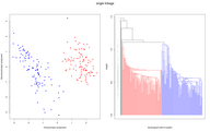
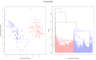
and for the following graphics different hierarchical clustering methods were then used. Each graphic consists of two parts:

• The left part shows the first two main components of the data. This representation is chosen because in this (two-dimensional) representation the distances in the surface correspond well to the distances in six-dimensional space. So if there are two clearly separated clusters (the distances between the clusters are large), one hopes to see them in this representation. The data points belonging to a cluster are marked with the same color; only with the black data points is it the case that each data point forms a cluster.
• In the right part we see the corresponding dendrogram. The "Height" on the y-axis indicates at which "distance" observations or clusters are combined to form a new cluster (according to the merging algorithm). If the two sub-clusters for a merger belong to the same cluster, the dendrogram is drawn in the corresponding color of the cluster; if they belong to different clusters, the color black is used. The gray dots on the left in the dendrogram again indicate at what “distance” a fusion took place. In order to determine a good number of clusters, the largest possible gap is sought in the gray points. Because a large gap means that there will be a large distance between the clusters to be merged during the next merger.

• 

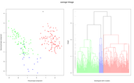
  Data and dendrogram for the average linkage method.

• 

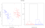
  Data and dendrogram using the Ward method.

• 

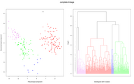
  Data and dendrogram for the complete linkage method.

• 

  Data and dendrogram for the single linkage method.

• 

  Data and dendrogram using the median method.

• 

  Data and dendrogram using the centroid method.

Divisive calculation

As mentioned above, there are theoretically possibilities to split a data set with objects into two parts. Divisive methods therefore normally need a heuristic in order to generate candidates who can then, for example, be evaluated using the same measures as in the agglomerative calculation. ${\displaystyle {\mathcal {O}}(2^{n})}$ ${\displaystyle n}$

Kaufman and Rousseeuw (1990) describe a divisive clustering procedure (Diana) as follows:

1. Start with a cluster that contains all the observations.
2. Calculate the diameter of all the clusters. The diameter is the maximum distance or dissimilarity of all objects within the cluster.
3. The cluster with the largest diameter is divided into two clusters.
4. For this purpose, the object in the cluster is determined which has the greatest average distance or dissimilarity to all other objects. It forms the core of the "splinter group".
5. Every object that is closer to the splinter group than the rest of the objects is now assigned to the splinter group.
6. Steps 2–5 are repeated until all clusters contain only one object.

Another special algorithm is the spectral relaxation .

See also

• Cluster analysis
• Data mining
• Knowledge Discovery in Databases
• Classification

literature

Basics and procedures

• M. Ester, J. Sander: Knowledge Discovery in Databases. Techniques and Applications. Springer, Berlin, 2000.
• K. Backhaus, B. Erichson, W. Plinke, R. Weiber: Multivariate analysis methods. Jumper
• S. Bickel, T. Scheffer, Multi-View Clustering. Proceedings of the IEEE International Conference on Data Mining, 2004.
• J. Shi, J. Malik: Normalized Cuts and Image Segmentation. in Proc. of IEEE Conf. on Comp. Vision and Pattern Recognition, Puerto Rico 1997.
• L. Xu, J. Neufeld, B. Larson, D. Schuurmans: Maximum margin clustering. In: Advances in Neural Information Processing Systems. 17 (NIPS * 2004), 2004

application

• J. Bacher, A. Pöge, K. Wenzig: Cluster analysis - application- oriented introduction to classification methods. 3. Edition. Oldenbourg, Munich 2010, ISBN 978-3-486-58457-8 .
• J. Bortz: Statistics for social scientists. (Chapter 16, cluster analysis). Springer, Berlin 1999.
• W. Härdle, L. Simar: Applied Multivariate Statistical Analysis. Springer, New York 2003.
• C. Homburg, H. Krohmer: Marketing Management: Strategy - Instruments - Implementation - Corporate Management. 3. Edition. Chapter 8.2.2, Gabler, Wiesbaden, 2009.
• H. Moosbrugger, D. Frank: Cluster analytical methods in personality research. An application-oriented introduction to taxometric classification methods . Huber, Bern 1992, ISBN 3-456-82320-7 .

Individual evidence

1. ↑ K. Florek, J. Łukasiewicz, J. Perkal, H. Steinhaus, S. Zubrzycki: Taksonomia wrocławska. In: Przegląd Antropol. 17, 1951, pp. 193-211.
2. ↑ K. Florek, J. Łukaszewicz, J. Perkal, H. Steinhaus, S. Zubrzycki: Sur la liaison et la division des points d'un ensemble fini. In: Colloquium Mathematicae. Vol. 2, No. 3-4, 1951, pp. 282-285. Institute of Mathematics Polish Academy of Sciences.
3. ↑ LL McQuitty: Elementary linkage analysis for isolating orthogonal and oblique types and typal relevancies. Educational and Psychological Measurement. 1957.
4. ^ PH Sneath: The application of computers to taxonomy. In: Journal of general microbiology. 17 (1), 1957, pp. 201-226.
5. ^ PNM Macnaughton-Smith: Some Statistical and Other Numerical Techniques for Classifying Individuals . Research Unit Report 6. London: Her Majesty's Stationary Office, 1965
6. ↑ ^{a b c} R. R. Sokal, CD Michener: A statistical method for evaluating systematic relationships . In: University of Kansas Science Bulletin 38 , 1958, pp. 1409-1438.
7. ^ JC Gower: A Comparison of Some Methods of Cluster Analysis. In: Biometrics 23.4, 1967, p. 623.
8. ↑ JH Ward Jr: Hierarchical grouping to optimize an objective function. In: Journal of the American statistical association. 58 (301), 1963, pp. 236-244.
9. ↑ R. Sibson: SLINK: an opti mally efficient algorithm for the single-link cluster method . In: The Computer Journal . tape 16 , no. 1 . British Computer Society, 1973, p. 30-34 ( http://www.cs.gsu.edu/~wkim/index_files/papers/sibson.pdf (PDF)).
10. ↑ D. Defays: An efficient algorithm for a complete link method . In: The Computer Journal . tape 20 , no. 4 . British Computer Society, 1977, pp. 364-366 .
11. ↑ Johannes Aßfalg, Christian Böhm, Karsten Borgwardt, Martin Ester, Eshref Januzaj, Karin Kailing, Peer Kröger, Jörg Sander, Matthias Schubert, Arthur Zimek: Knowledge Discovery in Databases, Chapter 5: Clustering . In: script KDD I . 2003 ( dbs.ifi.lmu.de [PDF]).
12. ↑ L. Kaufman, PJ Rousseeuw: Finding Groups in Data: An Introduction to Cluster Analysis . Wiley, New York 1990.