Fermi's golden rule

Fermi's Golden Rule , named after the physicist Enrico Fermi (1901–1954), describes a widely used equation from quantum mechanical perturbation theory . The equation gives the theoretical prediction for the transition rate ( the transition probability per time), with an initial state under the influence of a disturbance in a different state transitions . If transitions into other states are not possible, the reciprocal value of the transition rate indicates the mean service life of the initial state. Put clearly, this is the time that the quantum leap into the new state will on average still be a long time coming.

Due to its general validity, Fermi's Golden Rule can be used in a variety of ways, e.g. B. in atomic physics , nuclear physics and solid state physics for the absorption and emission of photons , phonons or magnons . The golden rule can be used to treat both spontaneous transformations (e.g. radioactive decay , the emission of light quanta , the decay of unstable elementary particles ) and absorption (e.g. of light quanta), but also the cross-section of any reactions between two particles .

formula

If an initial state is exposed to a perturbation through which it can change into a final state in an energy continuum , then in a first perturbative approximation the transition rate (i.e. the transition probability per unit of time) is given by ${\displaystyle |i\rangle }$ ${\displaystyle V}$ ${\displaystyle |f\rangle }$ ${\displaystyle \lambda _{i\to f}}$

${\displaystyle \lambda _{i\to f}={\frac {2\pi }{\hbar }}\rho (E_{f})\left|V_{fi}\right|^{2}}$

Are there

• ${\displaystyle \hbar }$the reduced Planck quantum of action
• ${\displaystyle \rho (E_{f})}$the density of states of the observed final states for the energy ${\displaystyle E_{f}}$
• ${\displaystyle V_{fi}}$the matrix element of the perturbation operator belonging to this transition , also expressed by . ${\displaystyle V}$ ${\displaystyle \langle f|V|i\rangle }$
• the states and eigen-states of an undisturbed Hamilton operator , in addition to which the disturbance is to be considered. ${\displaystyle |i\rangle }$ ${\displaystyle |f\rangle }$ ${\displaystyle V}$

The transition rate has the dimension 1 / time. For spontaneous decays (example: radioactivity ) it is the decay constant in the exponential law. The mean life of the system in the initial state is

${\displaystyle \tau =1/\lambda }$

The energy uncertainty or half width

${\displaystyle \Gamma _{i\to f}=\hbar \cdot \lambda _{i\to f}}$

the initial state has the dimension of energy.

If conversions in different forms are possible, the total decay constant or the total half width result from the sum of the individual partial values ​​for each type of transition. ${\displaystyle \lambda }$ ${\displaystyle \Gamma }$

history

The perturbation-theoretical formalism of the “Golden Rule” was developed by Paul Dirac in 1927 in order to treat the absorption and emission of photons for the first time in a quantum-mechanical way. In the thesis, the interaction (disturbance) of a quantum system, for example an atom or molecule, with electromagnetic dipole radiation is presented, with the disturbance operator occurring here in contrast to the above model example in the form of a vector quantity , the so-called transition dipole moment. ${\displaystyle {\vec {M}}_{fi}}$

A little later it was developed again by Gregor Wentzel in a work on the calculation of the transition probability for the (radiationless) Auger-Meitner effect in atoms, which is also a transition from a discrete state in the atom to the continuous range of the spectrum. This “rule” is named after Fermi because he named it “Golden Rule No.” in a nuclear physics textbook in 1950. 2 ”listed. In the literature, however, the terms Wentzel-Fermi Golden Rule and Fermi-Wentzel Golden Rule are sometimes found .

Fermi describes the use of the second order term in perturbation theory for those transitions that would be forbidden according to the first order as the Golden Rule No. 1 .

Derivation sketch

As a basic assumption, a time-constant system with an exactly solvable Hamilton operator is extended by a perturbation operator . ${\displaystyle H_{0}}$ ${\displaystyle V}$

${\displaystyle H=H_{0}+V}$

Fermi's Golden Rule applies to any constant or time-dependent perturbation operator. They can represent the interaction with an external (constant or time-dependent) field or an additional type of interaction between the particles of the system that was not taken into account in (e.g. the possibility of generating a photon). The derivation for a time-constant perturbation operator is shown here. ${\displaystyle \,H_{0}}$

For the completed Hamilton operator the time-dependent Schrödinger equation

${\displaystyle \mathrm {i} \hbar \partial _{t}\left|\Psi (t)\right\rangle =H\left|\Psi (t)\right\rangle }$

be solved. At the beginning ( ) the system should be in a state of its own . The function you are looking for is developed according to the eigenfunctions of the undisturbed Hamiltonian (with energy eigenvalues ) and you have time-dependent coefficients: ${\displaystyle t=0}$ ${\displaystyle H_{0}}$ ${\displaystyle \left|\Psi (t)\right\rangle }$ ${\displaystyle \left|\Psi _{n}\right\rangle }$ ${\displaystyle E_{n}}$

${\displaystyle \left|\Psi (t)\right\rangle =\sum _{n=0}^{\infty }a_{n}(t)\,\left|\Psi _{n}\right\rangle \,e^{-{\frac {\mathrm {i} E_{n}t}{\hbar }}}}$.

The initial condition is everyone else . ${\displaystyle a_{i}(0)=1}$ ${\displaystyle a_{n}(0)=0}$

After inserting the Hamilton operator and wave function into the Schrödinger equation, the coefficient comparison yields:

${\displaystyle \mathrm {i} \hbar \,\partial _{t}a_{f}(t)=\sum _{n=0}^{\infty }V_{fn}\,a_{n}(t)\,e^{\mathrm {i} \omega _{fn}t}}$,

where an abbreviation for represents and applies. ${\displaystyle \omega _{fn}}$ ${\displaystyle {\tfrac {E_{f}-E_{n}}{\hbar }}}$ ${\displaystyle V_{fn}=\left\langle \Psi _{f}\right|V\left|\Psi _{n}\right\rangle }$

This equation describes how the coefficients change over time. For an approximate solution, it is assumed that the coefficients change continuously compared to their initial values, so that only the term of the sum is to be considered for small times . (That is the sense of the first perturbative approximation.) Since is constant over time, the equation can be integrated: ${\displaystyle a_{f}(t)}$ ${\displaystyle n=i}$ ${\displaystyle V_{fi}}$

${\displaystyle \mathrm {i} \hbar a_{f}(t)=V_{fi}\int _{0}^{t}\mathrm {d} t'\,e^{\mathrm {i} \omega _{fi}t'}}$

The result is

${\displaystyle \mathrm {i} \hbar a_{f}(t)=V_{fi}\,{\frac {1}{\mathrm {i} \omega _{fi}}}\,(e^{\mathrm {i} \omega _{fi}t}-1)=2V_{fi}\;e^{\frac {\mathrm {i} \omega _{fi}t}{2}}\,\left({\frac {\sin {\tfrac {\omega _{fi}t}{2}}}{\omega _{fi}}}\right)}$.

It should be remembered that due to the derivation, this formula can only remain valid as long as it applies. The probability of finding the system in state f at time t is the square of the absolute value ${\displaystyle \left|a_{f}(t)\right|\ll 1}$

${\displaystyle \left|a_{f}(t)\right|^{2}={\frac {4\left|V_{fi}\right|^{2}}{\hbar ^{2}}}\left({\frac {\sin ^{2}{\tfrac {\omega _{fi}t}{2}}}{\omega _{fi}^{2}}}\right)}$.

With a transition into the continuum, the end state has numerous neighboring states with a similar structure, but with continuously varying energy, which are also possible as end states. The matrix element can therefore be assumed to be the same for all; However, the respective transition probability is different because of the factor in brackets (marked with in the following graphic ) in the last formula. Depending on considered, this factor is a function with an acute maximum of the height at . The neighboring zeros are included , the maximum in between can be easily approximated by a triangle with the base line . The average of the clamp factor in this interval is, therefore, approximately half of the maximum . ${\displaystyle f}$ ${\displaystyle g}$ ${\displaystyle \omega _{fi}}$ ${\displaystyle g}$ ${\displaystyle {\tfrac {t^{2}}{4}}}$ ${\displaystyle \omega _{fi}=0}$ ${\displaystyle \omega _{fi}=\pm {\tfrac {2\pi }{t}}}$ ${\displaystyle {\tfrac {4\pi }{t}}}$ ${\displaystyle {\tfrac {t^{2}}{8}}}$

The central maximum of the transition probability distribution (in any units). The height of the maximum centered at is proportional to , while the width is proportional to . ${\displaystyle E_{i}=E_{f}}$ ${\displaystyle t^{2}}$ ${\displaystyle {\tfrac {1}{t}}}$

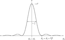
The peak maximum of this function at shows that transitions preferentially lead to states of the same energy , but deviations in a range of width are possible. This fluctuation range becomes smaller with increasing time. This is one of the forms of the uncertainty relation for energy and time and justifies the natural line width that can be found in all spectral lines . Also, with increasing t, the peak becomes higher, and the total area below the maximum (approximated by half the height times the width) increases proportionally to t . If W is the sum of the transition probabilities in all states in the region of the maximum, then W grows proportionally to t , and is the constant transition rate sought. But let me repeat that the whole derivation can only remain valid as long as it remains. ${\displaystyle \omega _{fi}=0}$ ${\displaystyle E_{f}=E_{i}}$ ${\displaystyle \Delta E={\tfrac {4\pi \hbar }{t}}={\tfrac {2h}{t}}}$ ${\displaystyle {\tfrac {W}{t}}}$ ${\displaystyle W\ll 1}$

To calculate W , the mean transition probability at the maximum is now simply multiplied by the number of end states in the interval . This number of states results from the density of states on the energy axis ${\displaystyle \Delta E}$

${\displaystyle \rho (E_{f})={\frac {\mathrm {d} n}{\mathrm {d} E_{f}}}}$

multiplied by the width . It should be noted that the density of states of all possible states in the energy interval is not necessarily as it is e.g. B. is defined in solid state physics, but mostly only a small fraction of it. Only those states contribute here that are also included in the concrete measurement of the transition probability , e.g. B. only those where particles fly in certain directions. ${\displaystyle \Delta E={\tfrac {4\hbar \pi }{t}}}$ ${\displaystyle \rho (E)}$ ${\displaystyle D(E)}$ ${\displaystyle E\pm {\tfrac {1}{2}}\Delta E}$ ${\displaystyle W}$

This gives the sum W of all individual transition probabilities ${\displaystyle \left|a_{f}(t)\right|^{2}}$

${\displaystyle W={\frac {4\left|V_{fi}\right|^{2}}{\hbar ^{2}}}\left({\frac {t^{2}}{8}}\right)\left({\frac {4\hbar \pi }{t}}\right)\rho (E_{f})\ =\ {\frac {2\pi }{\hbar }}\;\rho (E_{f})\;\left|V_{fi}\right|^{2}\;t}$.

Division by time gives Fermi's Golden Rule for the transition rate:

${\displaystyle \lambda _{i\to f}={\frac {2\pi }{\hbar }}\rho (E_{f})\left|V_{fi}\right|^{2}}$

literature

Because of its importance for quantum mechanical perturbation theory, Fermi's Golden Rule is covered in most introductory books on quantum mechanics.

• H. Haken, HC Wolf: Molecular Physics and Quantum Chemistry . 5th edition. Springer, Berlin, Heidelberg 2006, ISBN 978-3-540-30314-5 , pp. 322-327 .
• A. Amann, U. Müller-Herold: Open quantum systems . Springer, Berlin, Heidelberg 2011, ISBN 978-3-642-05186-9 , pp. 208-233 .
• T. Mayer-Kuckuk: Atomic Physics . 5th edition. BG Teubner, Stuttgart 1997, ISBN 978-3-519-43042-1 , p. 129-133 .
• JJ Sakurai: Modern Quantum Mechanics . Addison-Wesley, 1994, ISBN 0-201-53929-2 .
• W. Greiner: Quantum Mechanics Part I - An Introduction . 4th edition. Harry Deutsch, Thun 1989, ISBN 978-3-8171-1064-3 .

Web links

• Transition Probabilities and Fermi's Golden Rule
• Detailed derivation (PDF, English; 117 kB)
• Free Matlab code to visualize the rule

Remarks

1. ↑ Why it is referred to as a “rule” instead of “equation” or “formula” as is usually the case is not clear. In any case, this word can be reminiscent of the early days of the new quantum mechanics, when it was still necessary to try out which recipes or rules lead to success.

Individual evidence

1. ^ Paul Dirac The Quantum Theory of the Emission and Absorption of Radiation , Proceedings Royal Society A, Volume 114, 1927, p. 243
2. ^ Gregor Wentzel: About radiationless quantum leaps . In: Journal of Physics . tape 43 , no. 8 , 1927, pp. 524-530 , doi : 10.1007 / BF01397631 .
3. ^ Enrico Fermi: Nuclear Physics . University of Chicago Press, 1950, pp. 142 .
4. ↑ Fermi, loc. cit. P. 136