
Contingency table
Contingency tables (also: contingency tables or crosstabs ) are tables that contain the absolute or relative frequencies ( frequency tables ) of combinations of certain characteristics. Contingency means that two characteristics appear together. This means that there are frequencies for each other by multiple "and" or ", and" ( conjunction ) associated features shown. These frequencies are supplemented by their marginal sums, which form the so-called marginal frequencies . The frequent special case of a contingency table with two characteristics is a confusion matrix .
Structure and application
In contrast to a normal ( "flat") table that has these attributes in the 1st line attribute name and in all other rows forms, in a cross table both row and column headings characteristic values , and at the intersection of the respective column and row a value is shown that depends on the characteristics specified in the respective column and row.
| \ | Edge frequency of |
||||
|---|---|---|---|---|---|
| Edge frequency of |


A general crosstab for two variables and is shown on the right. The characteristics of the variables and the variables are given above and on the left. The number of occurrences and can be different for both variables. If it is the same, one speaks of square cross tables.


The table shows the absolute frequencies , i.e. H. the number of observations in which both the characteristic expression and occurs. The marginal frequencies are shown on the right and the marginal frequencies below .


Finally, at the bottom right is the sum of the marginal frequencies
,

where is the number of observations in the data set.

Instead of absolute frequencies, relative frequencies can also be displayed. In this case, instead of is used often and of course it applies .


Four-field table
A four-field table is a special form of a two-dimensional contingency table. Both variables have only two characteristics and they are structured as follows:
feature total total


Example of a two-dimensional contingency table
2000 people are asked whether they prefer product A or B. The result is evaluated according to the gender of the respondent. The following four-field table results
- with absolute frequencies
Product \ gender Female male total Product A 660 340 1000 Product B 340 660 1000 total 1000 1000 2000
- with relative frequencies based on the number of cases
Product \ gender Female male total Product A 0.33 0.17 0.5 Product B 0.17 0.33 0.5 total 0.5 0.5 1
- with relative frequencies based on the columns
Product \ gender Female male total Product A 0.66 0.34 1 Product B 0.34 0.66 1 total 1 1
- with relative frequencies based on the rows
Product \ gender Female male total Product A 0.66 0.34 1 Product B 0.34 0.66 1 total 1 1
Appearances can be deceptive
At first glance, it can be seen that female customers tend towards product A, while male customers tend towards product B. This can be interesting information - but it can also just be a fallacy. The evaluation of the survey with regard to the age of the customers shows:
Product \ age up to 40 years over 40 years total Product A 700 300 1000 Product B 300 700 1000 total 1000 1000 2000
Buying behavior therefore depends not only on gender, but also on the age of the respondents. The need to bring both information about dependencies into a realistic relationship to one another forces the development of a three-dimensional contingency table.
In order to be able to infer properties of the underlying populations from the relationships in the examined samples , chi-square tests can be used (under certain conditions) . The exact Fisher test is a statistical test of independence in contingency for small samples.
Categories to be used in contingency tables
In particular, the statistical procedures, which are based on contingency tables, place requirements on the categories (a single characteristic value or a combination of different characteristic values):
- Strictly speaking, all categories must be completely independent of one another. For example, a person cannot be “female” and “male” at the same time (except in rare cases of intersex , which are neglected here); but with “attended elementary school” and “completed apprenticeship” you can actually include the members of the latter group in the first - as attendance at elementary school is mandatory for everyone (in western societies). The problem is that the marginal frequencies do not then add to or add up.
- Furthermore, there should be no rows or columns in the contingency table in which the frequencies add up to zero. For example, such a panel cannot have the categories “male” and “female” when examining an exclusively male or exclusively female population. The problem is that the reciprocal of this sum occurs in the static evaluation and 1/0 is not defined.
- In addition, a “Other” category should be used as rarely as possible; for example as in “drives Opel”, “drives Peugeot”, “drives Toyota”, “drives another passenger car”. If it becomes necessary, this “collecting pot” should be kept as small as possible through a well thought-out concept.

Three-dimensional contingency table
For a three-dimensional table (three characteristics), additional columns are added to the table:
Gender Female Gender Male Product \ age up to 40 years over 40 years up to 40 years over 40 years total Product A 630 (70%) 30 (30%) 70 (70%) 270 (30%) 1000 Product B 270 (30%) 70 (70%) 30 (30%) 630 (70%) 1000 total 900 (100%) 100 (100%) 100 (100%) 900 (100%) 2000
The percentages added in brackets are only intended to draw attention to the fact that product propensity was in no way dependent on gender: 70% of younger women as well as men and 30% of older women as well as men are equally inclined to product A; with product B it is exactly the opposite.
To make this phenomenon more plausible, it may be worthwhile to look at a (this time again two-dimensional) contingency table:
Gender \ age up to 40 years over 40 years total Female 900 100 1000 Male 100 900 1000 total 1000 1000 2000
It becomes clear here that an overwhelming majority of 90% were female among the younger respondents. The younger customers prefer product A - not the female ones! On the other hand, older people (mainly men in the survey) prefer product B. The gender ratio in the example is only an apparent ratio that could arise due to the unbalanced statistical amount.
Graphical representation
3D bar charts are ideal for the graphic representation of two-dimensional contingency tables. A disadvantage of such diagrams, however, is that bars can be covered depending on the perspective. In addition, the 3-D display introduces a perspective that can make it difficult for the viewer to compare the height of the bars with one another in order to see which cell contains more observations.
Another option that is particularly useful for contingency tables with relatively few cells is a stacked bar chart that relates to the relative column frequencies.
It is better to use a mosaic plot in which the areas correspond to the frequencies for each combination of characteristic values. In addition, the independence of two or more variables can easily be displayed.
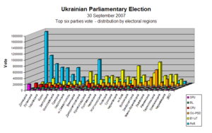
3D bar chart of the results of the parliamentary elections in Ukraine on September 30, 2007, broken down by regions and parties.

Stacked column chart referring to relative column frequencies (fictitious data).

Mosaic plot of the frequencies of passengers on the Titanic according to the variables class (1st class, 2nd class, 3rd class, crew), gender (male, female) and survived (yes, no).
.PNG)


statistical evaluation
As the contingency tables become more complex, relationships can no longer be read off simply with the eye. Statistics use a number of methods for systematic analysis:
- Relationship measures:
- Contingency Coefficient : -Coefficient, (corrected) Contingency Coefficient, Cramérs V and Phi Coefficient
- Error reduction measures : Goodman and Kruskals λ and τ as well as the uncertainty coefficient
- Testing:
- Further analysis methods:

See also
- Simpson's paradox
- Four-field correlation , four-field test for the simplest case
Individual evidence
- ↑ Heiner Abels: Handbook of the statistical diagram: construction, interpretation and manipulation of graphic representations (German edition) . Verlag Neue Wirtschafts-Briefe, 1981, ISBN 978-3-482-56581-6 .
Web links
- Video on the crosstab ( WMV ; 19.6 MB)