
Logistic equation
The logistic equation was originally introduced in 1837 by Pierre François Verhulst as a demographic mathematical model. The equation is an example of how complex, chaotic behavior can arise from simple nonlinear equations. As a result of a pioneering work by the theoretical biologist Robert May in 1976, it found widespread use. As early as 1825 Benjamin Gompertz presented a similar equation in a related context.
The associated dynamics can be illustrated using a so-called fig tree diagram (see below). The Feigenbaum constant, found by Mitchell Feigenbaum in 1975, plays an important role in this .
The demographic model
For the continuous case see logistic function .
Mathematical laws are sought that represent the development of a population in a model manner. From the size of the population at a certain point in time , conclusions should be drawn about the size after a reproductive period (e.g. after a year).


The logistic model takes two influences into account:
- The population increases geometrically through reproduction . The number of individuals in the following year is one growth factor larger than the current population.
- By starving the population decreased. The number of individuals decreases depending on the difference between their current size and a theoretical maximum size with the proportionality constant . So the factor by which the population decreases is the shape .


In order to take both processes into account when calculating the population in the following year, the current population is multiplied by both the multiplication factor and the hunger factor . This gives the logistic equation

- .

To simplify the following mathematical studies, the population size is often given as a fraction of the maximum size :

- .

In addition , and are combined into the parameter :

- .

This results in the following notation for the logistic equation:

Here is the capacity of the biotope. That is, it is the population which, with a suitable choice of the fixed point, corresponds to the dynamics.

The mathematical model
For results


is a number between and . It represents the relative size of the population in the year . The number therefore stands for the starting population (in year 0). The parameter is always positive, it reflects the combined effect of reproduction and starvation.


Behavior depending on r
The animation below shows the time series development of the logistic equation in the time and frequency domain ( Fourier analysis ) for .


The zones of intermittency within the deterministic chaos are clearly visible .
At various , the following behaviors can be observed for major ones. This behavior does not depend on the initial value, but only on :
- With from 0 to 1 the population dies out in any case.
- With 1-2, the population approaches monotonically the limit on.
- With 2-3, the population approaches the limit alternately, d. H. From a certain point on, the values are alternately above and below the limit value.
- With between 3 and (about 3.45) the sequence changes for almost all start values (except 0, 1 and ) between the two surroundings of two accumulation points .
- With between and approximately 3.54, the sequence changes between the surroundings of four accumulation points for almost all starting values.
- If it becomes greater than 3.54, first 8, then 16, 32 etc. accumulation points appear. The intervals with the same number of accumulation points ( bifurcation intervals) are getting smaller and smaller; the length ratio of two successive bifurcation intervals approaches the fig tree constant . This constant is also important in other mathematical contexts. (Numerical value: δ ≈ 4.6692016091029906718532038204662016172581 ...).
- The chaos begins at approximately 3.57 : The sequence initially jumps periodically between the surroundings of the now unstable accumulation points. As it grows, these intervals merge in such a way that their number halves in the rhythm of the fig tree constant until there is only one interval in which the sequence is chaotic. Periods are then no longer recognizable. Tiny changes in the initial value result in a wide variety of subsequent values - a property of chaos.
- For many coefficients between 3.57 and 4, chaotic behavior occurs, although for certain again there are cluster points (i.e. stable periodic orbits to which almost every initial value converges). For example, there are first 3, then 6, 12 etc. accumulation points in the vicinity of increasing . There are also r values with 5 or more accumulation points - all periods appear.
- Three deep-seated mathematical theorems state the following: (1) every interval of coefficients, no matter how small, contains parameters for which there are stable periodic orbits (so that the dynamics are not chaotic): non-chaotic parameters are "dense" in the interval of the Coefficients. Chaotic parameters therefore do not contain any intervals. But (2) the chaotic parameters have a positive dimension: that is, with a really positive probability, a random parameter delivers chaotic dynamics. Finally (3) almost every real coefficient (in the sense of full probability) either has a stable periodic orbit (to which almost every initial value converges) or is in the strict sense "chaotic". (There are other dynamic possibilities, but they have zero probability.)
- For more than 4, the sequence diverges for almost all initial values and leaves the interval .


![[0; 1]](https://wikimedia.org/api/rest_v1/media/math/render/svg/bc3bf59a5da5d8181083b228c8933efbda133483)
This transition from convergent behavior via period doubling to chaotic behavior is generally typical for nonlinear systems that show chaotic or non-chaotic behavior depending on a parameter.
An extension of the range of values to the complex numbers leads to the Mandelbrot set after a coordinate transformation .
example
The “logistic curve” with a growth rate is S-shaped. From a value of around 3.6, chaos breaks out, as the figure illustrates.


Graphical representation
The following bifurcation diagram , known as the Feigenbaum diagram , summarizes these observations. The horizontal axis indicates the value of the parameter and the vertical axis the accumulation points for the sequence .
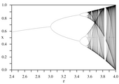
Logistic equation bifurcation diagram
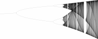
High resolution version without scale

High-resolution section of the bifurcation diagram of the logistic equation


Relationship with the Mandelbrot set (after coordinate transformation)

Analytical solution
There is an analytical solution for the parameter :


Analytical solutions can also be specified for the parameters and .


Individual evidence
- ^ Pierre-François Verhulst: Notice sur la loi que la population suit dans son accroissement. In: Correspondance Mathématique et Physique. Volume 10, 1838, ZDB ID 428605-4 , pp. 113-121.
- ^ Robert May: Simple mathematical models with very complicated dynamics Nature V. 261, pp. 459-467 (June 10, 1976)
- ^ Benjamin Gompertz: On the Nature of the Function Expressive of the Law of Human Mortality, and on a New Mode of Determining the Value of Life Contingencies. In: Philosophical Transactions of the Royal Society of London. Vol. 115, 1825, ISSN 0260-7085 , pp. 513-585.
- ↑ Jürgen Beetz: 1 + 1 = 10. Mathematics for cavemen. Springer, Heidelberg 2012, ISBN 978-3-8274-2927-8 , p. 313 f.
Web links
- Eric W. Weisstein. "Fig Tree Constant." From MathWorld - A Wolfram Web Resource.
- Analytical solution for the parameters -2, 2, 4
- Online calculation of the bifurcation diagram
- Java program of the chair for physics and its didactics at the University of Würzburg for the visualization of the logistic equation