Amount of almond bread

Amount of Mandelbrot (black) with a colored area. A complex number is assigned to each pixel . The number of iterations required is color-coded so that . It increases by 1 from color strip to color strip. ${\displaystyle c}$ ${\displaystyle n}$ ${\displaystyle z_{n+1}=z_{n}^{2}+c}$ ${\displaystyle |z_{n}|>10^{3}}$

The Mandelbrot set , named after Benoît Mandelbrot , is the set of complex numbers for which the iteration ${\displaystyle c}$

${\displaystyle {\begin{aligned}z_{0}&=0\\z_{n+1}&=z_{n}^{2}+c\end{aligned}}}$

defined sequence is limited . ${\displaystyle (z_{n})_{n\in \mathbb {N} }}$

Geometrically interpreted as part of the Gaussian plane of numbers, the Mandelbrot set is a fractal that is often called the apple man in common parlance . Images of this can be generated by placing a pixel grid on the number plane and thus assigning a value of to each pixel . If the sequence is restricted with the corresponding one , i.e. it belongs to the Mandelbrot set, the pixel is z. B. colored black, and otherwise white. If, instead, the color is determined according to how many sequence elements have to be calculated until it is certain that the sequence is not restricted, a so-called speed image of the Mandelbrot set is created: the color of each pixel indicates how quickly the sequence with the relevant one strives towards infinity . ${\displaystyle c}$ ${\displaystyle c}$ ${\displaystyle c}$

The first computer graphic representations were presented in 1978 by Robert Brooks and Peter Matelski . In 1980 Benoît Mandelbrot published a paper on the subject. It was later systematically examined by Adrien Douady and John Hamal Hubbard in a series of fundamental mathematical works. The mathematical basis for this was worked out in 1905 by the French mathematician Pierre Fatou .

Mandelbrot amount, different representation

definition

The Mandelbrot set (black) in the complex plane

Definition via recursion

The Mandelbrot set is the set of all complex numbers for which the recursively defined sequence of complex numbers with the formation law ${\displaystyle \mathbb {M} }$ ${\displaystyle c}$ ${\displaystyle z_{0},z_{1},z_{2},\dotsc }$

${\displaystyle z_{n+1}=z_{n}^{2}+c}$

and the initial term

${\displaystyle z_{0}=0}$

remains limited . That is, a complex number is an element of the Mandelbrot set if the amounts calculated with this do not exceed every limit, regardless of how large it becomes. This can be written as follows: ${\displaystyle c}$ ${\displaystyle \mathbb {M} }$ ${\displaystyle c}$ ${\displaystyle z_{n}}$ ${\displaystyle n}$

${\displaystyle z_{0}=0,z_{n+1}=z_{n}^{2}+c;\;\;c\in \mathbb {M} \iff \exists g\in \mathbb {R} :\limsup _{n\to \infty }|z_{n}|\leq g}$.

One can easily show that the amount that increases over any limit when a occurs with , so this definition is synonymous with: ${\displaystyle z_{n}}$ ${\displaystyle z_{n}}$ ${\displaystyle |z_{n}|>2}$

${\displaystyle z_{0}=0,z_{n+1}=z_{n}^{2}+c;\;\;c\in \mathbb {M} \iff \limsup _{n\to \infty }|z_{n}|\leq 2}$.

Definition via complex quadratic polynomials

The Mandelbrot set can also be described using complex quadratic polynomials:

${\displaystyle P_{c}:\mathbb {C} \to \mathbb {C} ,\,z\mapsto z^{2}+c}$

with a complex parameter . For each there will be the consequence ${\displaystyle c}$ ${\displaystyle c}$

${\displaystyle (P_{c}^{0}(0),\;P_{c}^{1}(0),\,P_{c}^{2}(0),\,\dotsb )=(\,P_{c}^{n}(0)\,)_{n\in \mathbb {N} }}$

iteratively calculated, where the -fold means the iteration is carried out one after the other, i.e. ${\displaystyle P_{c}^{n}}$ ${\displaystyle n}$

${\displaystyle P_{c}^{0}(z)=z}$

${\displaystyle P_{c}^{n+1}(z)=P_{c}(P_{c}^{n}(z)),\;n\in \mathbb {N} }$.

Depending on the value of the parameter , this sequence is either unlimited, so that it is not an element of the Mandelbrot set, or it remains within a range around the origin of the number level and is an element of the Mandelbrot set. ${\displaystyle c}$ ${\displaystyle c}$ ${\displaystyle c}$

The Mandelbrot set is a subset of the complex numbers with the definition

${\displaystyle \mathbb {M} =\lbrace c\in \mathbb {C} \;|\;\exists s\in \mathbb {R} :\forall n\in \mathbb {N} :|P_{c}^{n}(0)|\leq s\rbrace }$

or equivalent

${\displaystyle \mathbb {M} =\lbrace c\in \mathbb {C} \;|\;\forall n\in \mathbb {N} :|P_{c}^{n}(0)|\leq 2\rbrace }$

Some properties and examples are given for explanation:

• Based on the previously described statement, it can be set. The value indicates the radius around the origin within which an element of can lie. Outside of this circle no elements of can be found. ${\displaystyle s=2}$ ${\displaystyle s=2}$ ${\displaystyle \mathbb {M} }$ ${\displaystyle \mathbb {M} }$
• Because of the absolute value function, it is symmetrical to the real axis. ${\displaystyle \mathbb {M} }$
• In order to display the amount graphically, the values ​​of the parameter must all be calculated individually up to a self-determined number of iterations. ${\displaystyle \mathbb {M} }$ ${\displaystyle c}$
• Is that the consequence and is limited. Hence is element of . ${\displaystyle c=-2}$ ${\displaystyle 0,-2,2,2,2,2,\dotsc }$ ${\displaystyle c=-2}$ ${\displaystyle \mathbb {M} }$
• For the iterative sequence shows divergence and is not an element of . ${\displaystyle c=2}$ ${\displaystyle 0,2,6,38,\dotsc }$ ${\displaystyle c=2}$ ${\displaystyle \mathbb {M} }$

Definition via Julia sets

The Mandelbrot set was originally introduced by Benoît Mandelbrot to classify Julia sets , which were studied by the French mathematicians Gaston Maurice Julia and Pierre Fatou at the beginning of the 20th century . The Julia set for a certain complex number is defined as the boundary of the set of all initial values for which the above number sequence remains restricted. It may prove to be that the Mandelbrot set exactly the set of values is, for the corresponding Julia set coherently is. ${\displaystyle \mathbb {M} }$ ${\displaystyle J_{c}}$ ${\displaystyle c}$ ${\displaystyle z_{0}}$ ${\displaystyle \mathbb {M} }$ ${\displaystyle c}$ ${\displaystyle J_{c}}$

This principle is deepened in many results on the behavior of the Mandelbrot set . Shishikura shows that the edge of the Mandelbrot set , like the corresponding Julia set, has Hausdorff dimension 2. An unpublished manuscript by Jean-Christophe Yoccoz served John Hamal Hubbard as the basis for his results on locally connected Julia sets and locally connected Mandelbrot sets . ${\displaystyle \mathbb {M} }$ ${\displaystyle \mathbb {M} }$ ${\displaystyle J_{c}}$ ${\displaystyle J_{c}}$ ${\displaystyle \mathbb {M} }$

Geometric and mathematical properties

Play media file

Animation: Zoom into a crowd of Mandelbrot

The Mandelbrot set is closed (since its complement is open) and contained in the closed disk with radius 2 around the origin and is therefore compact .

If and denotes the -th iteration, then a point belongs to the Mandelbrot set if and only if ${\displaystyle P_{c}(z)=z^{2}+c}$ ${\displaystyle P_{c}^{n}(z)}$ ${\displaystyle n}$ ${\displaystyle c}$

${\displaystyle |P_{c}^{n}(0)|\leq 2}$ for all ${\displaystyle n\geq 0.}$

If the amount is greater than 2, the point escapes to infinity during iteration and therefore does not belong to the Mandelbrot set. ${\displaystyle P_{c}(0)}$

The enormous variety of shapes in the Mandelbrot set is evident from their relationship to Julia sets . Julia sets for iteration are fractals, except for some values ​​like (distance) or (circle). The shapes of these fractal structures are always the same within a Julia set, but span an enormous wealth of shapes for different parameters for Julia sets . It turns out that the structures of the Mandelbrot set in the vicinity of a certain value exactly reflect the structures of the associated Julia set . The Mandelbrot set thus contains the complete wealth of forms of the infinitely many Julia sets ( see below ). ${\displaystyle z\to z^{2}+c}$ ${\displaystyle c}$ ${\displaystyle c=-2}$ ${\displaystyle c=0}$ ${\displaystyle c}$ ${\displaystyle c}$ ${\displaystyle J_{c}}$

In the fractal structures at the edge there are scaled-down approximate copies of the entire Mandelbrot set, the satellites. Each image section of the Mandelbrot set that includes points from as well as points outside of contains an infinite number of these satellites. Almost the same structures occur immediately at the edge of a satellite as in the corresponding places on the original. However, towards the outside, these structures are combined with the structures that are typical for the larger environment of the satellite. ${\displaystyle \mathbb {M} }$ ${\displaystyle \mathbb {M} }$

Since each satellite is in turn equipped with satellites of a higher order, it is always possible to find a point at which any number of any different structures can be combined in any order. However, these structures can only be seen at extreme magnification.

The Mandelbrot set is mirror-symmetric to the real axis. It is contiguous (that is, it does not form islands), as demonstrated by Adrien Douady and John Hamal Hubbard in 1984, and it is speculated (Douady / Hubbard) that it is locally contiguous (MLC conjecture). This is one of the big open questions in the complex dynamics and so far unproven (although there are partial results, for example from Jean-Christophe Yoccoz , who proved the local connection for certain values ​​of , for the finitely renormalisable points). The MLC allows far-reaching conclusions about the topology of the Mandelbrot set. For example, the hyperbolicity conjecture would follow from this that every open set in the Mandelbrot set (i.e. the interior of the Mandelbrot set) consists of points with attractive cycles. The Mandelbrot set is self-similar , but not exact, because no two substructures of its edge are exactly alike; but in the vicinity of many edge points periodic structures form with continued enlargement of the section. At certain points the set of Mandelbrot has self-similarity (suggested by John Milnor and proven by Mikhail Lyubich 1999). ${\displaystyle c}$

Since the Mandelbrot set contains cardioid and circular areas, it has the fractal dimension 2. The edge of the Mandelbrot set has an infinite length, and its Hausdorff dimension , according to the work of Mitsuhiro Shishikura, is also 2; this implies that the box dimension has the value 2. It is conceivable that the edge of the Mandelbrot set has a positive (necessarily finite) area; otherwise this area would be zero. The area of ​​the Mandelbrot set is not known and, according to numerical estimates, is about 1.5065918849.

The Mandelbrot set contains deformed copies of all Julia sets, as Tan Lei proved in 1990 for the Misiurewicz points of the Mandelbrot set that lie close to the edge of the Mandelbrot set. This is further evidence of the close relationship between the structure of Julia and Mandelbrot sets. Thus, in the proofs of Yoccoz for the local connection of the Mandelbrot set at finitely renormalizable points, and Shishikura on the fractal dimension of the edge of the Mandelbrot set, the corresponding properties of the Julia sets belonging to the parameter value were first examined and then transferred to the Mandelbrot set.

The question of whether the Mandelbrot set is decidable makes no sense at first, since it is uncountable . The Blum-Shub-Smale model represents an approach to generalize the concept of decidability to uncountable sets . Within this model , the Mandelbrot set cannot be decided. ${\displaystyle \mathbb {M} }$

Picture gallery of a zoom ride

The following exemplary sequence of images of a zoom drive to a certain point gives an impression of the wealth of geometric shapes and explains certain typical structural elements. The magnification in the last picture is about 1 in 60 billion. In relation to a normal computer screen, this section behaves like the total size of the Mandelbrot set of 2.5 million kilometers, the edge of which in this resolution shows an unimaginable abundance of various fractal structures. ${\displaystyle c}$

image description Start picture: The amount of Mandelbrot with a continuously colored outside area. Section 1: Gap between “head” and “body”, called “Valley of the Seahorses”. Section 2: left double spirals, right “seahorses”. Section 3: "Seahorses". The “body” is formed by 25 “spokes”, of which two groups of twelve can be traced back to one of the two “fingers” on the “upper hand” of the set of Mandelbrot in the manner of a metamorphosis . The number of “spokes” therefore increases by two from one “seahorse” to the next. The "hub" is formed by a Misiurewicz point (see below). A deformed satellite can be seen between the “upper body” and “tail”. Section 4: The "seahorse's tail" also ends in a Misiurewicz point . Section 5: Part of the “tail”. The only path that winds through the entire "tail" and thus ensures that it is simply connected, leads in a zigzag from one "tail side" to the other, passing the "hubs" of the large 25-spiral structures. ${\displaystyle \mathbb {M} }$ Section 6: satellite. The two "seahorse tails" form the prelude to a series of concentric wreaths with the satellite in the center. Section 7: Each of these wreaths consists of structural elements of the same type, the number of which per wreath increases by powers of 2, a typical phenomenon in the vicinity of satellites. The above-mentioned path through the "seahorse's tail" passes the satellite via the notch of the cardioids and the tip of the "antenna" on the "head".

image description Section 8: “Antenna” of the satellite. Several 2nd order satellites can be seen on it. Section 9: “Valley of the Seahorses” from the satellite. The same structural elements can be seen as in section 1. Section 10: double spirals and "seahorses", which, however, in contrast to section 2, are outwardly equipped with seahorse-like extensions. This phenomenon demonstrates the concatenation of structural elements typical of nth order satellites for the case . ${\displaystyle n+1}$ ${\displaystyle n=1}$ Section 11: double spirals with 2nd order satellites. They can be interpreted as a metamorphosis of the “antenna”. Section 12: In the area of ​​the outer projections, island-like structures are always interspersed, which resemble Julia sets J c . The largest in the picture can just be seen in the center of the "double hook" on the right. Section 13: Part of the "double hook". Section 14: At first glance, these islands seem to consist of an infinite number of incoherent parts in the manner of Cantor sets , as is actually the case for the associated J c , but here they are connected to one another via filigree structures. These structures are based on a satellite in the center, which is not yet visible at this magnification, in such a way that the whole thing results in a simply coherent structure. Of the corresponding J c corresponding value is not the center of the image, but has relative to Hauptkardioide the same position as the image center to the satellite, which is shown in segment. 7 ${\displaystyle c}$ Section 15: Details of an island. Detail 16: details of a spiral.

An animation for this zoom trip can be found on the web links .

Behavior of the sequence of numbers

The various structural elements of are closely related to certain behaviors of the number sequence on which they are based. Depending on the value of , there are four possibilities: ${\displaystyle \mathbb {M} }$ ${\displaystyle \mathbb {M} }$ ${\displaystyle c}$

• It converges towards a fixed point.
• It converges to a periodic limit cycle that consists of two or more values. This also includes the cases in which the sequence behaves periodically from the start.
• It never repeats itself, but it remains limited. Some values ​​show chaotic behavior with alternation between almost periodic limit cycles and apparently random behavior.
• It diverges towards infinity ( certain divergence ).

All values ​​that do not diverge definitely belong to . ${\displaystyle c}$ ${\displaystyle \mathbb {M} }$

The following table shows examples of these four limit behaviors of the iteration for : ${\displaystyle z_{n+1}=z_{n}^{2}+c}$ ${\displaystyle z_{0}=0}$

parameter	Followers ${\displaystyle z_{2},z_{3},z_{4},z_{5},\ldots }$	Boundary behavior
On the real axis ...
${\displaystyle c=-3}$	${\displaystyle 6,\,33,\,1086,\,1179393,\,\dotsc }$	certain divergence against ${\displaystyle +\infty }$
${\displaystyle c=-2}$	${\displaystyle 2,\,2,\,2,\,2,\,\dotsc }$	immediate convergence towards the fixed point ${\displaystyle 2}$
${\displaystyle c=-1{,}75}$	${\displaystyle {\tfrac {21}{16}},\,-{\tfrac {7}{256}},\,-{\tfrac {114639}{65536}},\,\dotsc }$	Convergence towards the triple limit cycle ${\displaystyle -1{,}74697\ldots ,\,1{,}30193\ldots ,\,-0{,}54958\ldots }$
${\displaystyle c=-1{,}5}$	${\displaystyle {\tfrac {3}{4}},\,-{\tfrac {15}{16}},\,-{\tfrac {159}{256}},\,-{\tfrac {73023}{65536}},\,\dotsc }$	chaotic behavior
${\displaystyle c=-1{,}4}$	${\displaystyle 0{,}56,\,-1{,}0864,\,-0{,}21973504,\,\dotsc }$	Convergence towards 32 limit cycle
${\displaystyle c=-1{,}25}$	${\displaystyle {\tfrac {5}{16}},\,-{\tfrac {295}{256}},\,{\tfrac {5105}{65536}},\,\dotsc }$	Convergence against alternating limit cycle ${\displaystyle -1{,}20710\ldots ,\,0{,}20710\ldots }$
${\displaystyle c=-1}$	${\displaystyle -1,\,0,\,-1,\,0,\,-1,\,0,\,\dotsc }$	instant convergence against alternating limit cycle ${\displaystyle -1,\,0}$
${\displaystyle c=-0{,}75}$	${\displaystyle -{\tfrac {3}{16}},\,-{\tfrac {183}{256}},\,-{\tfrac {15663}{65536}},\,\dotsc }$	very slow convergence towards the fixed point ${\displaystyle -{\tfrac {1}{2}}}$
${\displaystyle c=-0{,}5}$	${\displaystyle -{\tfrac {1}{4}},\,-{\tfrac {7}{16}},\,-{\tfrac {79}{256}},\,-{\tfrac {26527}{65536}},\,\dotsc }$	Convergence towards a fixed point ${\displaystyle {\tfrac {1}{2}}-{\sqrt {\tfrac {3}{4}}}}$
${\displaystyle c=-0{,}25}$	${\displaystyle -{\tfrac {3}{16}},\,-{\tfrac {55}{256}},\,-{\tfrac {13359}{65536}},\,\dotsc }$	Convergence towards a fixed point ${\displaystyle {\tfrac {1}{2}}-{\sqrt {\tfrac {1}{2}}}}$
${\displaystyle c=0}$	${\displaystyle 0,\,0,\,0,\,0,\,0,\,0,\,\dotsc }$	immediate convergence towards the fixed point ${\displaystyle 0}$
${\displaystyle c=+0{,}25}$	${\displaystyle {\tfrac {5}{16}},\,{\tfrac {89}{256}},\,{\tfrac {24305}{65536}},\,\dotsc }$	Convergence towards a fixed point ${\displaystyle {\tfrac {1}{2}}}$
${\displaystyle c=+1}$	${\displaystyle 2,\,5,\,26,\,677,\,458330,\,\dotsc }$	certain divergence against ${\displaystyle +\infty }$
In the complex number plane ...
${\displaystyle c=-i}$	${\displaystyle -1-i,\,i,\,-1-i,\,i,\,\dotsc }$	instant convergence against alternating limit cycle ${\displaystyle -1-i,\,i}$
${\displaystyle c=-{\tfrac {1}{8}}+{\tfrac {3}{4}}i}$	${\displaystyle -{\tfrac {43}{64}}+{\tfrac {9}{16}}i}$	Convergence towards the triple limit cycle

Mandelbrot set with color-coded period length of the limit cycles

Geometric assignment

Convergence is present precisely for the values ​​of which form the interior of the cardioids , the "body" of , as well as for countably many of their edge points. Periodic boundary cycles can be found in the (approximately) circular “buds” as in the “head”, in the cardioids of the satellites and also on the countable number of edge points of these components. A fundamental conjecture says that there is a limit cycle for all internal points of the Mandelbrot set. The sequence is genuinely pre-periodic for a countable number of parameters, which are often called Misiurewicz-Thurston points (after Michał Misiurewicz and William Thurston ). These include the "antenna tips" like the point on the far left and branch points of the Mandelbrot set. ${\displaystyle c}$ ${\displaystyle \mathbb {M} }$ ${\displaystyle z=-2}$

In the uncountably many other points of the Mandelbrot set, the sequence can behave in many different ways, each of which generates very different dynamic systems and which are in part the subject of intensive research. Depending on the definition of the word, “chaotic” behavior can be found.

Periodic behavior

The circular structures

Each circular “bud” and each satellite cardioid is characterized by a certain periodicity of the limit cycle towards which the sequence for the associated values ​​strives. The arrangement of the “buds” on the associated cardioid follows the following rules, from which the periodicities can be read directly. Each “bud” touches exactly one basic body, namely a larger “bud” or a cardioid. ${\displaystyle c}$

The periodicity of a “bud” is the sum of the periodicities of the next two larger “neighboring buds” in both directions on the same base body, if there are any. If there are only smaller "buds" at the edge of the base body up to the point of contact with its base body or up to the notch of the cardioid, instead of the periodicity of a "neighboring bud" that of the base body itself contributes to the total. The following properties can be derived directly from this:

• The “buds” or cardioids tend to be smaller, the greater their periodicity.
• The periodicity of the largest "bud" on a base body is always twice that of the " bun " with the period on the "head". ${\displaystyle 4}$
• The periodicity of a “bud” of a satellite is the product of the periodicity of the satellite cardioids and that of the corresponding “bud” of the main cardioids.

Furthermore, this rule explains the occurrence of certain sequences of “buds” such as from “head” to cardioid notch with an increase in periodicity to the next “bud” by the value or from “arm” to “head” by the value . ${\displaystyle 1}$ ${\displaystyle 2}$

Attractive cycles

If there is a sequence member with the property for one , then the sequence repeats itself strictly periodically from the beginning, namely with the period . Since by results -times application of the iteration, being squared at each step, it can be described as a polynomial of the degree formulate. The values ​​for periodic sequences of the period are therefore obtained from the zeros of this polynomial. It turns out that every sequence of numbers converges towards this cycle of numbers, provided that one of its sequence members comes close enough to this cycle, these are called attractors . This leads to the fact that all number sequences converge to a certain neighborhood of the value, which represents the attractor, towards a stable cycle of the period . Each circular “bud” and each cardioid of a satellite represents exactly one such environment. The areas with the periods to are listed as examples : ${\displaystyle c}$ ${\displaystyle z_{n}=z_{0}=0}$ ${\displaystyle n}$ ${\displaystyle z_{n}}$ ${\displaystyle n}$ ${\displaystyle c}$ ${\displaystyle 2^{n-1}}$ ${\displaystyle c}$ ${\displaystyle n}$ ${\displaystyle 2^{n-1}}$ ${\displaystyle c}$ ${\displaystyle n}$ ${\displaystyle 1}$ ${\displaystyle 3}$

• Period 1: The cardioids of the main male apple. The edge of this cardioid is given by points of the shape with . ${\displaystyle c={\tfrac {1}{2}}z-{\tfrac {1}{4}}z^{2}}$ ${\displaystyle |z|=1}$
• Period 2: The "head". The 2nd zero corresponds to the main cardioid, which naturally occurs as the zero when determining all higher periods because of the period . This consideration shows that the number of attractors with the period can be at a maximum , and that only if it is a prime number. The head itself is a circular disk with a center and a radius , i. That is, the edge of this circular disk is given by points of the shape with . ${\displaystyle c=0}$ ${\displaystyle 1}$ ${\displaystyle n>1}$ ${\displaystyle 2^{n-1}-1}$ ${\displaystyle n}$ ${\displaystyle -1}$ ${\displaystyle {\tfrac {1}{4}}}$ ${\displaystyle c=-1+{\tfrac {1}{4}}z}$ ${\displaystyle |z|=1}$
• Period 3: The “buds” that correspond to the “poor” and the cardioids of the largest satellite on the “head antenna”. The fourth zero is omitted again. ${\displaystyle c=0}$

The number of attractive cycles with the exact period , i.e. H. and is minimal with this property, the sequence is A000740 in OEIS . ${\displaystyle n}$ ${\displaystyle z_{n}=z_{0}}$ ${\displaystyle n}$

Gallery of iteration

The following gallery gives an overview of the values ​​of for some values ​​of . It depends on the parameter whose real part extends from left to right in the images from −2.2 to +1, and whose imaginary part ranges from −1.4 to +1.4. ${\displaystyle z_{n}}$ ${\displaystyle n}$ ${\displaystyle z_{n}}$ ${\displaystyle c}$

The iteration z → z² + c after n steps

Iterations description n = 1 applies after the first step . So the picture is a colored representation of the complex numbers that are in the area shown. The zero is shown in white and infinite in black. Therefore, the further away a point is from the origin, the darker it appears. The color of a point provides information about its argument , i.e. about the angle it has with the positive-real axis (red). The negative real axis is colored turquoise. ${\displaystyle z_{1}(c)=c}$ ${\displaystyle c}$ n = 2 after two steps ${\displaystyle z_{2}(c)=c^{2}+c=c\cdot (c+1)}$ This expression becomes zero for as well as for . The newly added left zero is in the center of the head of the Mandelbrot set, while the old one on the right is the heart of the body cycloids. ${\displaystyle c=0}$ ${\displaystyle c=-1}$ n = 3 The number of zeros has doubled - as after every iteration step. The real zero on the left is in the heart of the small antenna satellite. The first complex-valued zeros appear above and below the real axis. These zeros are in the center of each arm. n = 4 The bun was created: it belongs to the zero position to the left of the head zero position at −1. The function shown ${\displaystyle z_{4}(c)=\left((c^{2}+c)^{2}+c\right)^{2}+c}$ becomes more and more confusing. However, it can easily be checked that if a zero is from , then a zero is from . Therefore "inherits" the zeros from . This relationship is the reason for the periodic behavior of the buds explained below . ${\displaystyle c}$ ${\displaystyle z_{n}}$ ${\displaystyle c}$ ${\displaystyle z_{k\cdot n}}$ ${\displaystyle z_{4}}$ ${\displaystyle z_{2}}$

Iterations description n = 5 Since it is a prime number, there are no well-known zeros - except for the zero, which is known from the past. Since the degree of the polynomial is the same , it grows faster with increasing towards infinity. As a result, the edge between the amount of Mandelbrot and its exterior is becoming increasingly clear. ${\displaystyle 5}$ ${\displaystyle z_{1}}$ ${\displaystyle z_{n}(c)}$ ${\displaystyle 2^{n-1}}$ ${\displaystyle z_{n}}$ ${\displaystyle n}$ n = 9 In the meantime there are already zeros that are also distributed within the Mandelbrot set. Since there is a divisor of , the arm buds and the small antenna satellite are again on the line with a zero and therefore light up brightly. ${\displaystyle 256}$ ${\displaystyle 3}$ ${\displaystyle 9}$ n = 17 Again a prime number. n = 18 This series of images ends with and zeros. could be enlarged at will, which would increase the number of new buds. ${\displaystyle n=18}$ ${\displaystyle 2^{17}=131072}$ ${\displaystyle n}$

Using the series of images above, it can be seen for the iteration stage that the zero point is an inner point of . So it depends on the number of iterations whether there are zeros within or not. ${\displaystyle n=18}$ ${\displaystyle c=-1}$ ${\displaystyle \mathbb {M} }$ ${\displaystyle \mathbb {M} }$

Repulsive cycles

In addition to attractive cycles, there are repulsive ones, which are characterized by the fact that sequences of numbers in their environment are increasingly moving away from them. However, they can be achieved because, apart from the situation due to the square in the iteration rule , each has two potential predecessors in the sequence that differ only in their sign . Values ​​for which the associated sequence eventually leads to such an unstable cycle via such a second precursor of a period member are, for example, the "hubs" of the wheel or spiral structures as well as the end points of the widespread antenna-like structures, which are formally known as "hubs" be interpreted by “wheels” or spirals with a single spoke. Such values ​​are known as Misiurewicz points . ${\displaystyle z_{n}}$ ${\displaystyle z_{n-1}=0}$ ${\displaystyle c}$ ${\displaystyle c}$

A Misiurewicz point also has the property that in its immediate vicinity the associated Julia set is almost congruent with the same section . The closer the Misiurewicz point is, the better the agreement. Since Julia sets for values ​​are connected within and outside of Cantor sets made up of an infinite number of islands with a total area of ​​zero, they are particularly filigree in the transition zone at the edge of . Every Misiurewicz point is just a point on the edge of , and every section of the edge zone of , which contains points both inside and outside it, contains an infinite number of them. This represents the entire wealth of forms of all Julia sets of this filigree type in the area around the Misiurewicz points . ${\displaystyle c}$ ${\displaystyle \mathbb {M} }$ ${\displaystyle J_{c}}$ ${\displaystyle c}$ ${\displaystyle \mathbb {M} }$ ${\displaystyle \mathbb {M} }$ ${\displaystyle \mathbb {M} }$ ${\displaystyle \mathbb {M} }$ ${\displaystyle \mathbb {M} }$ ${\displaystyle \mathbb {M} }$ ${\displaystyle \mathbb {M} }$

Satellites

Analysis of the behavior of Newton's method for a family of cubic polynomials.

Another structural element that explains the wealth of forms in the Mandelbrot crowd are the scaled-down copies of themselves, which are found in the filigree structures of their edges. The behavior of the sequence of numbers within a satellite corresponds to that of the sequences in the main body in the following way. Within a satellite all sequences of numbers converge against limit cycles, the periods of which differ from those at the corresponding points in the main body by a factor . If only every -th sequence element is considered for a certain value from the satellite , then a sequence results which, apart from a spatial scale factor, is almost identical to that which results for the corresponding value in the main body of . The mathematical justification for this is profound; it comes from the work of Douady and Hubbard on "polynomial-like maps". ${\displaystyle \mathbb {M} }$ ${\displaystyle p}$ ${\displaystyle c}$ ${\displaystyle p}$ ${\displaystyle c}$ ${\displaystyle \mathbb {M} }$

The additional structural elements in the immediate vicinity of a satellite are a consequence of the fact that between two of the considered sequence members with the index spacing there can be one with the value that thus establishes a periodic course with the period . However, the corresponding sequence outside the main body diverges because it has no such intermediate links. ${\displaystyle p}$ ${\displaystyle z_{n}=0}$ ${\displaystyle n}$

The Mandelbrot set itself is a universal structure that can appear in completely different non-linear systems and classification rules. The basic prerequisite, however, is that the functions involved are angular . If systems that depend on a complex parameter are considered and their behavior is classified with regard to a certain property of the dynamics as a function of , then under certain circumstances small copies of the Mandelbrot set are found in the parameter level. One example is the question for which polynomials of the third degree the iterative Newton method for determining zeros with a certain starting value fails and for which it does not. ${\displaystyle c}$ ${\displaystyle c}$

As in the adjacent picture, the amount of Mandelbrot can appear distorted, for example the arm buds are in a slightly different place. Otherwise the amount of Mandelbrot is completely intact, including all buds, satellites, filaments and antennae. The reason for the appearance of the Mandelbrot set is that the considered function families in certain areas - apart from rotations and displacements - quite well with the function family

${\displaystyle \{f_{c}\colon z\mapsto z^{2}+c\mid c\in \mathbb {C} \}}$,

which defines the amount of Mandelbrot. Deviations are permitted to a certain extent, and yet the amount of Mandelbrot crystallizes out. This phenomenon is called structural stability and is ultimately responsible for the appearance of the satellites in the vicinity of , because partial sequences of the iterated functions locally show the same behavior as the entire family. ${\displaystyle \mathbb {M} }$

Intermediate changeable behavior

Representation of the amount of the sequence members as a function of the iteration step for a value with a particularly varied behavior of the sequence. The noticeable breaks in behavior result from almost catching in repulsive cycles, which temporarily leads to quasiperiodic behavior. ${\displaystyle n}$ ${\displaystyle c}$

Representation of the elements following the c value of the previous diagram as points in the complex plane with a stored Mandelbrot set for orientation. The brightness of a pixel is a measure of how many points in the sequence hit it.

Due to the possibility of the sequence of numbers to repeatedly get into the immediate vicinity of a repulsive cycle, and with the subsequently tending to divergent or chaotic behavior to almost get into another cycle, very complicated behavior patterns of the sequence can develop in the interim until the final character is formed the sequence shows how the two figures demonstrate. The environment of the associated values ​​in is correspondingly rich in structure. ${\displaystyle c}$ ${\displaystyle \mathbb {M} }$

The representation of the following points even in the complex level shows a greater complexity in these cases. The quasi-periodic behavior in the vicinity of a repulsive cycle often leads in these cases to spiral structures with several arms, with the following points circling the center while the distance to it increases. The number of arms therefore corresponds to the period. The point clusters at the ends of the spiral arms in the above figure are the result of the two associated near-catches by repulsive (unstable) cycles.

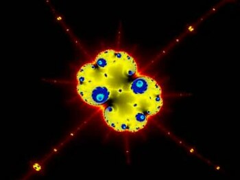
Density distribution of the sequence members

Accumulated density distribution of the sequence elements for all c values ​​in a color-coded representation

The picture on the right shows the density distribution of the sequence elements in the complex plane, which results from evaluating 60 million sequences, whereby the brightness is a measure of how many orbitals run through the point. Blue areas indicate sequential members with a low index, while yellowish areas indicate sequential members with high indexes. Sequences from the large cardioids of the Mandelbrot set tend to converge to a value on a circle around the origin, which can be seen as a round area with a very high density. The smaller structures near the imaginary axis mark the conjugate areas between which sequence elements of many sequences jump back and forth (approximation of a limit cycle with period 2 for large sequence indices). ${\displaystyle c}$

Relation to chaos theory

In the upper part of the picture, limit cycles of the logistic equation are shown, which correspond to real values ​​of the Mandelbrot set. Convergence turns into chaos via bifurcation . ${\displaystyle c}$

The law of formation on which the sequence is based is the simplest non-linear equation by means of which the transition from order to chaos can be provoked by varying a parameter. For this it is sufficient to consider real number sequences.

They are obtained when constraining to the values ​​of the axis of . For values , i.e. within the cardioids, the sequence converges. The sequence behaves chaotically on the “antenna” that extends up to . The transition to chaotic behavior now takes place via an intermediate stage with periodic limit cycles. The period increases gradually by a factor of two towards the chaotic area, a phenomenon known as period doubling and bifurcation . Each area for a certain period corresponds to one of the circular “buds” on the axis. ${\displaystyle c}$ ${\displaystyle x}$ ${\displaystyle \mathbb {M} }$ ${\displaystyle -0{,}75\leq c\leq 0{,}25}$ ${\displaystyle c=-2}$ ${\displaystyle c}$ ${\displaystyle x}$

The period doubling begins with the “head” and continues in the sequence of the “buds” to the “antenna”. The ratio of the lengths of successive parameter intervals and thus that of the bud diameter at different periods tends towards the Feigenbaum constant , a fundamental constant of chaos theory. This behavior is typical for the transition of real systems to chaotic dynamics. The noticeable gaps in the chaotic area correspond to islands with periodic behavior, to which the satellites on the "antenna" are assigned in the complex plane. ${\displaystyle \delta \approx 4{,}669}$

For certain complex values, limit cycles occur which lie on a closed curve, the points of which, however, are not covered periodically, but chaotically. Such a curve is known in chaos theory as a so-called strange attractor . ${\displaystyle c}$

The Mandelbrot set is therefore an elementary object for chaos theory, on which fundamental phenomena can be studied. For this reason it is occasionally compared with that of straight lines for Euclidean geometry with regard to its importance for chaos theory .

Graphic representation

The graphic representation of the Mandelbrot set and its structures in the edge area is only possible using a computer using so-called fractal generators . Each pixel corresponds to a value of the complex plane. For each pixel, the computer determines whether the associated sequence diverges or not. As soon as the amount of a sequence member exceeds the value , it is clear that the sequence is diverging. The number of iteration steps up to that point can serve as a measure of the degree of divergence. The pixel is colored according to a previously defined color table which assigns a color to each value . ${\displaystyle c}$ ${\displaystyle |z_{n}|}$ ${\displaystyle s=2}$ ${\displaystyle n}$ ${\displaystyle n}$

In order to achieve harmonious boundaries between successive colors from an aesthetic point of view, in practice not the smallest possible value is chosen for the boundary , but a value significantly greater than , since otherwise the width of the color strip oscillates. The larger this value is chosen, the better the color boundaries correspond to equipotential lines that result when the Mandelbrot set is interpreted as an electrically charged conductor . For continuous color gradients, as in the above zoom picture series, it is necessary to evaluate the factor by which it was exceeded when the value was exceeded for the first time. ${\displaystyle s}$ ${\displaystyle s=2}$ ${\displaystyle 2}$ ${\displaystyle s}$

Since the number of iteration steps after which the limit is exceeded for the first time can be as large as desired, a termination criterion in the form of a maximum number of iteration steps must be specified. Values ​​of , the consequences of which have not yet exceeded the limit afterwards , are included in the calculation. As a rule, the smaller the distance from zu , the larger the number after which it is exceeded. The greater the magnification with which the edge of is displayed, the greater the maximum number of iteration steps must be selected, and the more computing time is required. If it can be seen that the sequence converges for a start value , the calculation of the sequence can be terminated earlier. ${\displaystyle n}$ ${\displaystyle s}$ ${\displaystyle c}$ ${\displaystyle s}$ ${\displaystyle \mathbb {M} }$ ${\displaystyle c}$ ${\displaystyle \mathbb {M} }$ ${\displaystyle n}$ ${\displaystyle s}$ ${\displaystyle \mathbb {M} }$ ${\displaystyle c}$

The representation of the edge of with its wealth of forms is particularly attractive graphically . The greater the selected magnification, the more complex structures can be found there. With the appropriate computer programs , this edge can be displayed with any magnification, as with a microscope . The only two artistic freedoms that exist are the choice of the image section and the assignment of colors to the degree of divergence. ${\displaystyle \mathbb {M} }$

To examine interesting structures, magnifications are often required which cannot be calculated with hardware-supported data types due to their limited accuracy. Some programs therefore contain long number arithmetic data types with arbitrarily selectable precision. This means that (almost) any enlargement factors are possible.

Sample program

Iteration over all pixels

The following sample program assumes that the pixels of the output device can be addressed using coordinates x and y with a value range from 0 to xpixels-1 and ypixels-1 , respectively . The calculation of the complex numerical value c assigned to the pixel with the real part c _re and the imaginary part c _im is carried out by linear interpolation between (re_min, im_min) and (re_max, im_max).

The maximum number of iteration steps is max_iter. If this value is exceeded, the corresponding pixel is assigned to the set . The value of max_iter should be at least 100. In the case of a higher magnification, considerably larger values ​​are sometimes required for the correct representation of the structures and thus significantly longer computing times. ${\displaystyle \mathbb {M} }$

PROCEDURE Apfel (re_min, im_min, re_max, im_max, max_betrag_2: double,
                 xpixels, ypixels, max_iter: integer)
  FOR y = 0 TO ypixels-1
    c_im = im_min + (im_max-im_min)*y/ypixels

    FOR x = 0 TO xpixels-1
      c_re = re_min + (re_max-re_min)*x/xpixels

      iterationen = Julia (c_re, c_im, c_re, c_im, max_betrag_2, max_iter)
      farb_wert   = waehle_farbe (iterationen, max_iter)
      plot (x, y, farb_wert)
    NEXT

  NEXT
END PROCEDURE

Iteration of a pixel

The iteration from to for a point on the complex number plane takes place through the iteration ${\displaystyle n}$ ${\displaystyle n+1}$ ${\displaystyle c}$

${\displaystyle {\begin{matrix}z_{n+1}&=&z_{n}^{2}+c\end{matrix}}}$,

which is obtained by breaking down the complex number into its real part and imaginary part into two real calculations ${\displaystyle z}$ ${\displaystyle x}$ ${\displaystyle y}$

${\displaystyle {\begin{matrix}x_{n+1}&=&x_{n}^{2}-y_{n}^{2}+c_{x}\end{matrix}}}$

and

${\displaystyle {\begin{matrix}y_{n+1}&=&2x_{n}y_{n}+c_{y}\end{matrix}}}$

can be disassembled. Here we have used the following identity:

${\displaystyle {\begin{matrix}z^{2}=(x+\mathrm {i} y)^{2}=x^{2}+2\mathrm {i} xy+(\mathrm {i} y)^{2}=x^{2}+2\mathrm {i} xy+(-1)y^{2}=x^{2}-y^{2}+\mathrm {i} (2xy)\end{matrix}}}$

If the square of the magnitude of the (n + 1) th number given by

${\displaystyle {\begin{matrix}|z_{n+1}|^{2}&=&x_{n+1}^{2}+y_{n+1}^{2}&&\end{matrix}}}$

exceeds the value max_ amount_2 (at least 2 * 2 = 4), the iteration is aborted and the number of iteration steps that have taken place so far is used for the assignment of a color value. If the square of the amount has not exceeded the max_ amount_2 after a given maximum number of iteration steps , it is assumed that the iteration remains restricted and the iteration loop is terminated.

The following function performs the iteration described. x and y are the iteratively used variables for the iteration values; xx, yy, xy and remain_iter are auxiliary variables.

 FUNCTION Julia (x, y, xadd, yadd, max_betrag_2: double, max_iter: integer): integer
   remain_iter = max_iter
   xx = x*x
   yy = y*y
   xy = x*y
   betrag_2 = xx + yy

   WHILE (betrag_2 <= max_betrag_2) AND (remain_iter > 0)
     remain_iter = remain_iter - 1
     x  = xx - yy + xadd
     y  = xy + xy + yadd
     xx = x*x
     yy = y*y
     xy = x*y
     betrag_2 = xx + yy
   END

   Julia = max_iter - remain_iter
 END FUNCTION

If a more continuous color gradient is desired, the formula is an alternative

    Julia = max_iter - remain_iter – log(log(betrag_2) / log(4)) / log(2)

which delivers real values ​​rather than whole. For the sequence with c  = 0 and the starting value z ₀  =  2 , this formula returns the value zero. This also results in a coloring that is independent of max_ amount_2 , provided this value is greater than 1.

A considerable part of the computing time is required where the sequence of numbers does not diverge. Modern programs try to reduce the computing time for these positions with various methods. One possibility is to abort the calculation when the sequence of numbers has converged or has caught up in a periodic cycle. Other programs take advantage of the fact that every point inside a closed curve, which only contains points from , also belongs to it. ${\displaystyle \mathbb {M} }$

Changing the data structure can also save computing time and even simplify the algorithm. In the following example, calculations with complex matrices are carried out with the NumPy program library , which means that there is no explicit iteration over all pixels.

import numpy as np
import matplotlib.pyplot as plt

d, n = 100, 50  # Pixeldichte & Anzahl der Iterationen
r = 2.5  # Fluchtradius (muss größer als 2 sein)

x = np.linspace(-2.5, 1.5, 4 * d + 1)
y = np.linspace(-1.5, 1.5, 3 * d + 1)

A, B = np.meshgrid(x, y)
C = A + B * 1j

Z = np.zeros_like(C)
T = np.zeros(C.shape)

for k in range(n):
    M = abs(Z) < r
    Z[M] = Z[M] ** 2 + C[M]
    T[M] = k + 1

plt.imshow(T, cmap=plt.cm.twilight_shifted)
plt.savefig("mandelbrot.png", dpi=200)

Computer-generated landscape of an island in the shape of the Mandelbrot set, rendered with the Terragen program .

Reception in public

Outside of the professional world, the Mandelbrot crowd was primarily known for the aesthetic value of the computer graphics , which is supported by the artistic color design of the outside area, which does not belong to the crowd. Through the publication of images in the media at the end of the 1980s, it achieved an unusually high level of awareness for a mathematical topic of this kind and is likely to be the most popular fractal, possibly the most popular object in contemporary mathematics.

The Mandelbrot set is said to be the geometrical structure with the most shape. It has inspired computer artists and contributed to the rise of fractal concepts. Numerous modifications of the algorithm on which the Mandelbrot set is based are used.

Another aspect is the extreme contrast between this and the simplicity of the underlying algorithm, which is reminiscent of biological systems, in which, from a scientific point of view, extremely complex systems can also arise from a comparatively small number of rules, as well as the proximity to chaos research , which also had aroused great public interest.

The name 'apple man' is derived from the rough geometric shape of a quantity of Mandelbrot rotated 90 degrees clockwise.

The American musician Jonathan Coulton has published a song about the Mandelbrot crowd, in which Benoît Mandelbrot is thanked for bringing order to the chaos.

Calculation speed

In the state of the art in the late 1980s, calculations took a long time. In comparison, this shows a list by the number of iterations that different CPUs could perform per second.

CPU	Accuracy (software)	Speed in iterations / sec	Computation time for 8.8 billion iterations
Z80 @ 1.75 MHz	32 bit floating point (1.)	9	31 years
Z80 @ 2.45 MHz	32 bit integer (2.)	280	01 year
80386 SX / 20 + IIT 3C87SX / 20	32 bit integer (3.)	130,000	19 hours
	80 bit floating point (FPU) (3.)	75,000	33 hours
	80 bit floating point (Borland emulation) (3.)	2,000	51 days
Pentium 90	32 bit integer (3.)	1,450,000	01 hour 40 minutes
	80 bit floating point (3.)	2,900,000	50 minutes
2 × Xeon E5-2623 v3	32 bit floating point (4.)	50,000,000,000	0.177 seconds
	64 bit floating point (4.)	25,000,000,000	0.35 seconds

Software used

1. BASIC interpreter
2. Assembler
3. Borland C ++ with integrated assembler
4. Visual Studio C ++ with Intel Intrinsics , use of AVX2 and fused multiply-add , multithreaded , 2 threads per core

literature

• Benoît Mandelbrot : The fractal geometry of nature. ISBN 3-7643-2646-8 .
• John Briggs, F. David Peat: The Discovery of Chaos. ISBN 3-446-15966-5 .
• Heinz-Otto Peitgen , Peter H. Richter: The Beauty of Fractals. ISBN 0-387-15851-0 .
• Heinz-Otto Peitgen, Dietmar Saupe: The Science of Fractal Images. ISBN 0-387-96608-0 .
• Karl Günter Kröber: The fairy tale of the apple man - 1. Paths to infinity. ISBN 3-499-60881-2 .
• Karl Günter Kröber: The fairy tale of the apple man - 2nd journey through the Malumite universe. ISBN 3-499-60882-0 .
• Dierk Schleicher: On Fibers and Local Connectivity of Mandelbrot and Multibrot Sets, in: M. Lapidus, M. van Frankenhuysen (eds): Fractal Geometry and Applications: A Jubilee of Benoît Mandelbrot. Proceedings of Symposia in Pure Mathematics 72, American Mathematical Society (2004), 477-507, 1999, pdf

Web links

Commons : Mandelbrot set  - collection of images, videos and audio files

Wiktionary: Mandelbrot quantity  - explanations of meanings, word origins, synonyms, translations

• Eric W. Weisstein : Mandelbrot Set . In: MathWorld (English).
• The Encyclopedia of the Mandelbrot Set (English)
• Animations for zooming in the article here - up to 1024 × 768 pixels
• Video almond bulbs
• Robert Devaney: Unveiling the Mandelbrot Set. At: Plus.Maths.org.
• Various algorithms for calculating the amount of Mandelbrot on rosettacode.org.
• Mandelbrot zoom 10 ^ 227 (1080x1920)

References and comments

1. ^ Robert Brooks, J. Peter Matelski: The dynamics of 2-generator subgroups of PSL (2, C). In: Riemann surfaces and related topics: Proceedings of the 1978 Stony Brook Conference. In: Annals of Mathematics Studies. Volume 97, Princeton University Press, Princeton, NJ, 1981, pp. 65-71. PDF.
2. ^ Benoît Mandelbrot: Fractal aspects of the iteration of for complex . ${\displaystyle z\mapsto \lambda z(1-z)}$ ${\displaystyle \lambda ,z}$In: Annals of the New York Academy of Sciences. 357, 249-259.
3. ^ Adrien Douady, John H. Hubbard: Etude dynamique des polynômes complexes. In: Prépublications mathémathiques d'Orsay. 2/4, 1984/1985 (PDF; 4.88 MB).  ( Page no longer available , search in web archives )  Info: The link was automatically marked as defective. Please check the link according to the instructions and then remove this notice.  
4. ↑ Robert P. Manufo: Escape radius. At: mrob.com. November 19, 1997.
5. ^ Lei Tan: Similarity between the Mandelbrot set and the Julia sets. In: Communications in Mathematical Physics. 1990, Vol. 134, No. 3, pp. 587-617. PDF. At: ProjectEuclid.org.
6. ^ Mitsuhiro Shishikura: The Hausdorff dimension of the boundary of the Mandelbrot set and Julia sets. March 1998, Vol. 147, No. 2, pp. 225-267. On-line. At: JStor.org.
7. ^ John H. Hubbard: Local connectivity of Julia Sets and bifurcation loci. Three theorems of J.-C. Yoccoz. Hubbard in his paper on page 511 cites an unpublished manuscript by J.-C. Yoccoz. PDF. 1993.
8. ↑ Numerical estimation of the area of ​​the Mandelbrot set (2012), online
9. ↑ After a corresponding coordinate transformation. For details see the picture description.
10. ^ Peitgen, Jürgens, Saupe: Chaos, building blocks of order. Rowohlt, ISBN 3-499-60551-1 , p. 431.
11. ↑ Jonathan Coulton: Mandelbrot set. ( Memento of the original from January 25, 2017 in the Internet Archive ) Info: The archive link was inserted automatically and has not yet been checked. Please check the original and archive link according to the instructions and then remove this notice. 

This version was added to the list of articles worth reading on October 13, 2005 .