Marching squares

Schematic representation of the algorithm: The gray squares are data values ​​on a grid . The isoline for an iso value in the dark gray value range is shown in red .

Marching Squares (from English "marching squares") is an algorithm from computer graphics for calculating isolines from a data source. Isolines are lines that connect data points with the same values.

Some typical applications for marching squares are the visualization of isobars on weather maps and level lines in altitude fields . The name of the algorithm is derived from how it works. The data set is broken down into square grid cells, which are processed one after the other. Marching Squares is related to the Marching Cubes algorithm, which is used to visualize isosurfaces . Marching Squares is used in 2D space and Marching Cubes in 3D space.

functionality

After the iso value has been determined for which the line is to be calculated, the data must be rasterized into a grid , unless the data set is already on a uniform grid. The data set can then be divided into a coarser grid. The cells of this coarse grid are stepped through.

For each grid cell it is checked whether its corner points are above or below the iso value. There can be 16 cases, which, taking symmetries into account, can be traced back to the following four:

• Case 1: all corners larger / smaller
• Case 2: exactly one corner larger / smaller
• Case 3: exactly two corners with a common edge larger / smaller
• Case 4: exactly two opposite corners larger / smaller

In the 4th case it cannot be decided how the two isoline segments should run through the cell. To do this, the inside of the cell must be examined.

• 

  Case 1 : All corners are above (or below) the iso value.

• 

  Case 2 : Except for one corner, all corners are above (or below) the iso value.

• 

  Case 3 : Two corners on each edge are above or below the iso value.

• 

  Case 4 : Two opposite corners are above or below the iso value.

• 

  Solution for case 4 depending on values ​​within the cell.

• 

  Solution for case 4 depending on values ​​within the cell.

If the isoline is to be scanned more finely than the rough grid allows, the grid cell can be subdivided again in cases 2 to 4 and the algorithm can be used repeatedly.

Edges with one end node above the iso value and the other below it are intersected by the isoline. The cutting position can be interpolated linearly , as the iso value and the values at the end nodes are known. The following applies to the calculation: with ${\displaystyle I}$ ${\displaystyle f_{i}}$ ${\displaystyle p_{i}=(x,y)}$ ${\displaystyle I=a\cdot f_{1}+b\cdot f_{2}}$ ${\displaystyle a+b=1}$

The cutting position is then . ${\displaystyle p_{I}=a\cdot p_{1}+b\cdot p_{2}}$

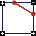
example

An object is bypassed here. There are 16 different options. In the illustration, the arrows point in the next direction to be approached.

swell

• Kai Hormann: Computergrafik 2. (PDF) June 22, 2006, accessed on September 5, 2009 . 
• Stefan Gumhold: Scientific visualization . Illustration. 2009 (lecture slides).

Web links

• Better know an Algorithm - Marching Square - A very good English guide
• All 16 configurations of one cell
• Implementation in Java