
Particle size distribution
The term particle size distribution is borrowed from statistics . There frequencies and frequency distributions of any feature, e.g. B. cube eyes, manufacturing tolerances, etc., considered. In the field of particle technology and particle measurement technology or dispersity analysis , the equivalent diameter of a particle is selected as the characteristic . The particle size distribution thus results from the general frequency distribution of the statistics. This is often referred to as the grain size distribution .
Definitions
The particles (disperse phase) within a surrounding medium (continuous phase), i.e. H. Grains, drops or bubbles are differentiated using an equivalent diameter to be measured and classified into selected classes according to their size. To represent a particle size distribution, the proportions with which the respective particle classes are involved in the disperse phase are determined.
Different types of quantities are used. If the particles are counted, the type of quantity is the number. In the case of weighing, however, it is the mass or, in the case of a homogeneous density ρ, the volume. Others are derived from lengths, projection and surfaces. One differentiates:
| Quantity type | Index r | Measurement method (examples) |
|---|---|---|
| number | 0 | electric mobility analysis |
| length | 1 | Sedimentation analysis |
| surface | 2 | Absorbance measurement |
| Volume (mass) | 3 | Sieve analysis |
A standardized quantity measure is used for the graphic representation. The normalization is necessary in order to eliminate the dependence of the proportions on the total amount used. In this way, for example, the result of a first weighing of 100 g total mass can be compared with the result of a weighing of 1 kg total mass.
A distinction is made between two quantities:
- Cumulative distribution Q r
- Density distribution q r
The terms Q r and q r are the symbols of the term quantile . The index r denotes the type of quantity according to the table above.
In general, when graphing a particle size distribution, the equivalent diameter x is plotted on the abscissa and the quantity Q r or q r on the ordinate .
Cumulative distribution curve
The cumulative distribution curve Q r (x) indicates the standardized amount of all particles with an equivalent diameter smaller than or equal to x . In the following, the cumulative distributions of the two most common types of quantities are explicitly defined:
- Particle number ( r = 0 )
- Let N i be the number of all examined particles with a diameter x smaller than or equal to the examined diameter x i and N the total number of all examined particles. Then

- Particle mass ( r = 3 )
- Let m i be the mass of all examined particles with a diameter x smaller than or equal to the examined diameter x i and m the total mass of all examined particles. Then

The same procedure is used for the other types of quantities.
Example : A weighing shows that 20 g of a sample with a total mass of 100 g fell through a sieve with a mesh size of 1 mm and is therefore smaller than 1 mm. thats why

Due to the normalization, i. H. the respective division by the total amount applies


The quantity Q r is always dimensionless.
The following diagram shows a typical cumulative distribution curve with the minimum and maximum equivalent diameters x min and x max . The discrete elements of the total distribution are plotted over the individual upper class limits x o, i :

Density distributions
Linear density distribution curve
If the difference between the quantitative proportions Q r of the equivalent diameter x u, i (lower limit of class i ) and x o, i (upper limit of class i), then the following applies:

The discrete density distribution q r (x) is thus defined as follows:

The following applies to the width of class i :

In the case of a differentiable cumulative distribution Q r (x) , the density distribution is the 1st derivative of Q r (x) :

The linear density distribution q r (x) has - provided x is an equivalent diameter - the unit [m −1 ]. The following diagram shows a typical density distribution curve:

The marked area is the proportion of the particles ΔQ r contained in the interval Δx i = x o, i - x u, i , the size or equivalent diameter x of which is between x u, i and x o, i . Due to the normalization of the cumulative distribution Q r , the area below the density distribution curve is equal to 1:

In practice, however, you will usually have to deal with discrete values , i.e. individual values, of the density distribution. The density distribution as a function is not explicitly known. Several possibilities of application are then used:
The density distribution is assumed to be constant in the interval Δx i . The result is a rectangular area:

Traverse :
The value of the density distribution q r for the interval (x u, i , x o, i ) is plotted at the location of the arithmetic class center , i.e. H. at x m, a = (x o, i + x u, i ) / 2 . The resulting data points are linearly connected as an approximation.
As with the polygon course, the value of the density distribution is plotted at the location of the arithmetic class center. The values are then connected by a polynomial approximation function (spline). It should be noted that the values interpolated in this way are of mathematical and not physical origin.
histogram

Traverse

Spline


The density distribution q r (x) very often shows the shape of a Gaussian bell. If the distribution only has a maximum, one speaks of a monomodal distribution. With two maxima the distribution is bimodal. The abscissa value of the greatest maximum is called the mode value.
Density function of the particle number concentration
In the field of atmospheric aerosols , the density function of the particle number concentration is used instead of the pure density function. For this purpose, the density distribution is multiplied by the measured particle number concentration.

The advantage of this form of representation is the direct comparability of particle size distribution and particle number concentration of aerosols.
Logarithmic density distribution (transformed density distribution)
The representation of a linear density distribution q r is impractical if the range of the available equivalent diameters extends over more than a decade. In this context, one speaks of a broad distribution. In these cases, it is advisable to use a logarithmically divided abscissa, as the overview is then much easier. The logarithmic density distribution is marked with q r * or q r, log . The value of the density distribution q r * for the interval (x u, i , x o, i ) is plotted at the location of the geometric class center , i.e. H. at:
![x _ {{m, i, g}} = {\ sqrt [{2}] {x _ {{o, i}} \ cdot x _ {{u, i}}}}](https://wikimedia.org/api/rest_v1/media/math/render/svg/e627ab4abb3be264b2fbdd8617d2f08ace96e0c3)
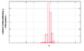
In practice, the logarithmic plot has often proven to be advantageous compared to the linear plot. The following diagram shows a logarithmic plot of a narrow distribution.

From a mathematical point of view, the logarithmic plot is a substitution of the abscissa. The following applies in general:

and with s = lg x = (ln x ) / 2.3026 one gets for the conversion

It must be emphasized that the logarithmic substitution of the abscissa leads to a change in the shape of the curve, i.e. H. among other things that the mode value shifts. The normalization condition, on the other hand, is always met.
literature
- DIN 66143 Representation of grain (particle) size distributions - power network. 1974.
- DIN 66144 Representation of grain (particle) size distributions - logarithmic normal distribution network. 1974.
- DIN 66145 representation of grain (particle) size distributions - RRSB network. 1976.
- DIN 66160 measurement of disperse systems, terms.
- DIN 66161 particle size analysis , symbols, units.
- DIN ISO 9276-1 Presentation of the results of particle size analyzes . Part 1: Graphic representation.
- Matthias Stieß: Mechanical process engineering. Volume 1. 2., revised edition. Springer, Berlin a. a. 1995, ISBN 3-540-59413-2 (3rd, completely revised edition, as: Mechanische Verfahrenstechnik. Volume 1: Partikeltechnologie. Ibid 2009 (published 2008), ISBN 978-3-540-32551-2 ).
- Albrecht F. Braun: The genetic interpretation of natural heaps with the help of the logarithmic grain network according to ROSIN, RAMMLER and SPERLING (DIN 4190). In: Journal of the German Geological Society. Vol. 126, 1975, ISSN 0012-0189 , pp. 199-205, abstract .