Edging

As Ränderung (ger .: Bordering Method ) a method of improving the solution properties are called linear equations . The method is used in linear algebra and numerics .

A system of linear equations

${\displaystyle Ax=b}$

with a singular or poorly conditioned system matrix , by adding rows and columns to and correspondingly enlarging and assigning an extended system of linear equations in which the system matrix is ​​well conditioned (i.e. also regular). The simple examples in the next two sections should clarify this. The system matrix supplemented by rows and columns is also known as a rimmed matrix . ${\displaystyle A\in \mathbb {R} ^{m\times n}}$ ${\displaystyle A}$ ${\displaystyle x}$ ${\displaystyle b}$

Example (regularization)

The system of equations is given

${\displaystyle (0)(x_{1})=(1)}$

with the system matrix , the ones vector of the unknowns and the right hand side . This can be regularized by changing the system matrix with the column and the row : ${\displaystyle 1\times 1}$ ${\displaystyle A=(0)}$ ${\displaystyle x=(x_{1})}$ ${\displaystyle b=(1)}$ ${\displaystyle \left({\begin{matrix}1\\0\end{matrix}}\right)}$ ${\displaystyle \left({\begin{matrix}1&0\end{matrix}}\right)}$

${\displaystyle \left({\begin{matrix}0&{\overline {1}}\\{\overline {1}}&{\overline {0}}\end{matrix}}\right)\left({\begin{matrix}x_{1}\\{\overline {x}}_{2}\end{matrix}}\right)=\left({\begin{matrix}1\\{\overline {0}}\end{matrix}}\right).}$

The entries added to the original system are overlined. The rimmed system has the unique solution with . Of this, the solution assigned to the original problem by the change is . The size of expresses how strong the regularizing influence of the change is. ${\displaystyle {\overline {x}}\in \mathbb {R} ^{2}}$ ${\displaystyle x_{1}=0,\;{\overline {x}}_{2}=1}$ ${\displaystyle x_{1}=0}$ ${\displaystyle {\overline {x}}_{2}}$

Example (improvement of fitness)

In this example, a measured value vector with 10% errors with respect to the Euclidean norm is assumed from the using the equation ${\displaystyle b\in \mathbb {R} ^{2}}$

${\displaystyle {\begin{matrix}\underbrace {\begin{pmatrix}1&10\\0&1\end{pmatrix}} &{\begin{pmatrix}x_{1}\\x_{2}\end{pmatrix}}&=&{\begin{pmatrix}b_{1}\\b_{2}\end{pmatrix}}&\\A\end{matrix}}}$

the sizes are to be determined. The solution results for For the right side deviating by approx. 10% (i.e. within the error tolerance)  , the completely different solution is determined . ${\displaystyle x_{1},x_{2}}$ ${\displaystyle b={\begin{pmatrix}1\\0\end{pmatrix}}}$ ${\displaystyle x={\begin{pmatrix}1\\0\end{pmatrix}}.}$ ${\displaystyle b={\begin{pmatrix}1\\0.1\end{pmatrix}}}$ ${\displaystyle x={\begin{pmatrix}0\\0.1\end{pmatrix}}}$

A measure of how strongly relative errors  in the measurement affect the relative error in  the calculation result is the condition of the system matrix  ${\displaystyle {\frac {|\Delta b|}{|b|}}}$ ${\displaystyle {\frac {|\Delta x|}{|x|}}}$ ${\displaystyle A}$

${\displaystyle \operatorname {cond} (A)=\max \left\{\left.{\frac {\frac {|\Delta x|}{|x|}}{\frac {|\Delta b|}{|b|}}}\;\right|\;b,\Delta b\in \mathbb {R} ^{n}\setminus \{0\},\;Ax=b,\;A(x+\Delta x)=(b+\Delta b)\right\}.}$

For the special choice of  from this example results  . Due to the poor condition of the matrix, relative errors in the measurement data  can be reflected  in the relative error of the values ​​calculated from these data  . ${\displaystyle A}$ ${\displaystyle \operatorname {cond} (A)\approx 102}$ ${\displaystyle b}$ ${\displaystyle A}$ ${\displaystyle x}$

This effect is graphically illustrated in the following image for the right-hand sides specified above. From the upper part of the image can be seen that the two column vectors and of are almost linearly dependent on each other. ${\displaystyle a^{(1)}:=\left({\begin{matrix}1\\0\end{matrix}}\right)}$ ${\displaystyle a^{(2)}:={\begin{pmatrix}10\\1\end{pmatrix}}}$ ${\displaystyle A}$

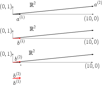
As a result, the two right-hand sides and , shown in red in the lower part of the image , which are very close to one another, fall into the image spaces of different columns from and the coefficients in ${\displaystyle b^{(1)}}$ ${\displaystyle b^{(2)}}$ ${\displaystyle A}$ ${\displaystyle x_{1},x_{2}}$

${\displaystyle a^{(1)}x_{1}+a^{(2)}x_{2}=Ax=b}$

differ from each other when switching from too much. ${\displaystyle b=b^{(1)}}$ ${\displaystyle b=b^{(2)}}$

Effect of a change: The addition of an additional line to corresponds to the expansion of the value range of by one dimension from to and with the addition of a column a new column vector is added. A clever choice of the additional components and the additional column vector ensures that the column vectors of the bordered matrix are separated from one another much better. More precisely, one chooses the new degrees of freedom so that the columns of the bordered matrix are perpendicular to each other and have the same length. ${\displaystyle A}$ ${\displaystyle A}$ ${\displaystyle \mathbb {R} ^{2}}$ ${\displaystyle \mathbb {R} ^{3}}$ ${\displaystyle {\overline {a}}^{(3)}}$ ${\displaystyle {\overline {a}}_{3}^{(1)},\;{\overline {a}}_{3}^{(2)}}$ ${\displaystyle {\overline {a}}^{(3)}}$ ${\displaystyle {\overline {A}}:=\left({\overline {a}}^{(1)}\;{\overline {a}}^{(2)}\;{\overline {a}}^{(3)}\right)}$ ${\displaystyle {\overline {a}}^{(1)},{\overline {a}}^{(2)},{\overline {a}}^{(3)}}$ ${\displaystyle {\overline {A}}}$

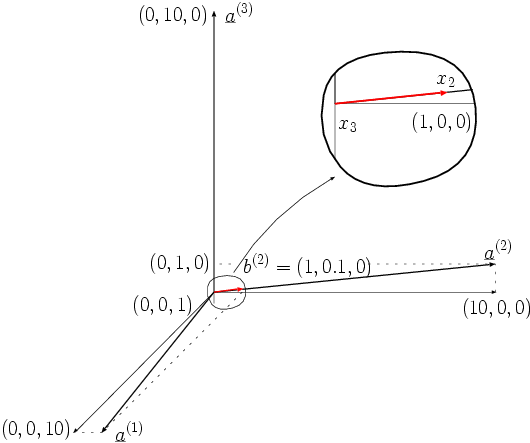
In the example, this is approximately achieved with the change

${\displaystyle {\underline {A}}:={\begin{pmatrix}1&10&{\underline {0}}\\0&1&{\underline {10}}\\{\underline {10}}&{\underline {0}}&{\underline {0}}\end{pmatrix}}.}$

The position of the column vectors in the bordered matrix is shown in the following figure. ${\displaystyle {\underline {A}}}$ ${\displaystyle \mathbb {R} ^{3}}$

For the modified system

${\displaystyle {\underline {A}}{\underline {x}}={\underline {b}}}$

result with the rimmed right-hand sides and the solutions and respectively  . The components essential for the measurement task and therefore do not change at all due to the 10% disruption of . ${\displaystyle {\underline {b}}^{(1)}=(1,0,0)}$ ${\displaystyle {\underline {b}}^{(2)}=(1,0.1,0)}$ ${\displaystyle {\underline {x}}^{(1)}=(0,0.1,-0.01)}$ ${\displaystyle {\underline {x}}^{(2)}=(0,0.1,0)}$ ${\displaystyle x_{1}}$ ${\displaystyle x_{2}}$ ${\displaystyle b}$

This is illustrated again in the following two images.

The condition number of the modified matrix has been reduced to. Calculating from the measured values ​​will only worsen the relative error by a maximum of approx. 15%. ${\displaystyle \operatorname {cond} ({\underline {A}})\approx 1.15}$ ${\displaystyle {\underline {x}}}$ ${\displaystyle {\underline {b}}}$

In this motivating example, the margins have been kept very simple. Through a skilful choice of Ränderung be reached that the relative error by calculating from no longer deteriorating, so that applies. ${\displaystyle x}$ ${\displaystyle b}$ ${\displaystyle \operatorname {cond} ({\underline {A}})=1}$

Regularization

Let be a real matrix and a matching -dimensional column vector. A rimmed matrix ${\displaystyle A}$ ${\displaystyle m\times n}$ ${\displaystyle b}$ ${\displaystyle m}$

${\displaystyle \left({\begin{matrix}A&A_{\rm {ro}}\\A_{\rm {lu}}&0\end{matrix}}\right)}$

with matching dies and is regular if the line from a base of the core form and the column of a minimal system of columns is that, together with the columns of the spans. In this case, the modified system ${\displaystyle A_{\rm {ro}}}$ ${\displaystyle A_{\rm {lu}}}$ ${\displaystyle A_{\rm {lu}}}$ ${\displaystyle A}$ ${\displaystyle A_{\rm {ro}}}$ ${\displaystyle A}$ ${\displaystyle \mathbb {R} ^{m}}$

${\displaystyle \left({\begin{matrix}A&A_{\rm {ro}}\\A_{\rm {lu}}&0\end{matrix}}\right)\left({\begin{matrix}x\\x_{u}\end{matrix}}\right)=\left({\begin{matrix}b\\0\end{matrix}}\right)}$

solve uniquely and is the dimension of the (square) bordered matrix (here is the defect of ). ${\displaystyle m+\operatorname {def} (A)}$ ${\displaystyle \operatorname {def} (A)}$ ${\displaystyle A}$

Depending on the choice of matrices and you can solve different tasks. If, for example, the rows of span the kernel of and the columns of the orthogonal complement of the image of , then the solution of the modified system of equations with the pseudo inverse of . The kernel of can be calculated with the help of the Gaussian elimination method and the orthogonal complement of the image of is conveniently calculated as the kernel of . ${\displaystyle A_{\rm {ro}}}$ ${\displaystyle A_{\rm {lu}}}$ ${\displaystyle A_{\rm {lu}}}$ ${\displaystyle A}$ ${\displaystyle A_{\rm {ro}}}$ ${\displaystyle A}$ ${\displaystyle x}$ ${\displaystyle A^{+}b}$ ${\displaystyle A^{+}}$ ${\displaystyle A}$ ${\displaystyle A}$ ${\displaystyle A}$ ${\displaystyle A^{T}}$

Optimal margins

The idea from the last section is taken up here and any matrix is modified in such a way that the columns of the expanded matrix are all perpendicular to one another and have the same Euclidean norm . The extended matrix is then the product of the largest singular value of with an orthogonal matrix and thus has the minimum possible condition number one. The representation used here is based on. ${\displaystyle A\in \mathbb {R} ^{m\times n}}$ ${\displaystyle {\overline {A}}}$ ${\displaystyle {\bar {A}}}$ ${\displaystyle A}$

Singular value decomposition as a tool for changing margins

The structure of the system matrix can be using one of the singular value decomposition of coordinate transformation gained , simplify. The new system matrix then has a large number of zero entries. Only the elements have non-zero elements, namely the singular values . Where is the rank of the matrix . ${\displaystyle A=U\Sigma V^{T}}$ ${\displaystyle A\in \mathbb {R} ^{m\times n}}$ ${\displaystyle b_{U}:=U^{T}b}$ ${\displaystyle x_{V}:=V^{T}x}$ ${\displaystyle \Sigma \in \mathbb {R} ^{m\times n}}$ ${\displaystyle \Sigma _{1,1},\ldots ,\Sigma _{r,r}}$ ${\displaystyle \Sigma _{1,1}:=\sigma _{1}\geq \Sigma _{2,2}:=\sigma _{2}\ldots \geq \Sigma _{r,r}:=\sigma _{r}>0}$ ${\displaystyle r}$ ${\displaystyle A}$

The transformation and are orthogonal and standard-sustaining , . From this it follows that the transformed system matrix has the same condition as the original system matrix . ${\displaystyle U\in \mathbb {R} ^{m\times m}}$ ${\displaystyle V\in \mathbb {R} ^{n\times n}}$ ${\displaystyle |b_{U}|=|U^{T}b|}$ ${\displaystyle |x_{V}|=|V^{T}x|}$ ${\displaystyle \Sigma }$ ${\displaystyle A}$

An extension

${\displaystyle {\bar {\Sigma }}:={\begin{pmatrix}\Sigma &{\bar {\Sigma }}_{\rm {ro}}\\{\bar {\Sigma }}_{\rm {lu}}&{\bar {\Sigma }}_{\rm {ru}}\end{pmatrix}}\in \mathbb {R} ^{{\bar {m}}\times {\bar {n}}}\qquad {\mbox{ mit }}{\bar {m}}\geq m{\mbox{ und }}{\bar {n}}\geq n}$

the matrix to matrix blocks (of mating dimensions) corresponds to a Ränderung the matrix when the transformation matrices and suitably by parts of the unit matrix adds: ${\displaystyle \Sigma }$ ${\displaystyle {\bar {\Sigma }}_{\rm {ro}}\in \mathbb {R} ^{{\bar {m}}\times ({\bar {n}}-n)},{\bar {\Sigma }}_{\rm {lu}}\in \mathbb {R} ^{({\bar {m}}-m)\times n},{\bar {\Sigma }}_{\rm {ru}}^{({\bar {m}}-m)\times ({\bar {n}}-n)}}$ ${\displaystyle A}$ ${\displaystyle U}$ ${\displaystyle V}$

${\displaystyle {\bar {A}}:={\begin{pmatrix}U&\mathbf {0} _{m\times ({\bar {m}}-m)}\\\mathbf {0} _{({\bar {m}}-m)\times m}&\mathbf {1} _{({\bar {m}}-m)\times ({\bar {m}}-m)}\end{pmatrix}}{\begin{pmatrix}\Sigma ^{(11)}&{\bar {\Sigma }}_{\mathrm {ro} }\\{\bar {\Sigma }}_{\mathrm {lu} }&{\bar {\Sigma }}_{\mathrm {ru} }\end{pmatrix}}{\begin{pmatrix}V^{T}&\mathbf {0} _{n\times ({\bar {n}}-n)}\\\mathbf {0} _{({\bar {n}}-n)\times n}&\mathbf {1} _{({\bar {n}}-n)\times ({\bar {n}}-n)}\end{pmatrix}}={\begin{pmatrix}U\Sigma V^{T}&U{\bar {\Sigma }}_{\mathrm {ro} }\\{\bar {\Sigma }}_{\mathrm {lu} }V^{T}&{\bar {\Sigma }}_{\mathrm {ru} }\end{pmatrix}}={\begin{pmatrix}A&U{\bar {\Sigma }}_{\mathrm {ro} }\\{\bar {\Sigma }}_{\mathrm {lu} }V^{T}&{\bar {\Sigma }}_{\mathrm {ru} }\end{pmatrix}}}$

The extended transformation matrices and are again orthogonal, so that the condition of the extended system matrix matches that of the matrix . ${\displaystyle {\bar {V}}:={\begin{pmatrix}V&\mathbf {0} \\\mathbf {0} &\mathbf {1} \end{pmatrix}}}$ ${\displaystyle {\bar {U}}:={\begin{pmatrix}U&\mathbf {0} \\\mathbf {0} &\mathbf {1} \end{pmatrix}}}$ ${\displaystyle {\bar {A}}}$ ${\displaystyle {\bar {\Sigma }}}$

In the following, only matrices need to be examined that have a system matrix with the structure (known from singular value decomposition)

${\displaystyle \Sigma _{i,j}=\left\{{\begin{matrix}\sigma _{i,i}&{\mbox{ wenn }}&i=j\leq r\\0&{\mbox{ sonst }}\end{matrix}}\right.}$

with an integer . ${\displaystyle 0\leq r\leq \min(m,n)}$

Completion of a rectangular matrix to a square one

Here only the modification of matrices with more rows than columns is described ( ). The statements can be transferred to matrices with more columns than rows by transposition. With the statements from the previous section it is clear that we are dealing with the study of matrices of form ${\displaystyle m>n}$

${\displaystyle \Sigma =\left({\begin{matrix}D\\\mathbf {0} \end{matrix}}\right)}$

where is a positive semidefinite diagonal matrix and a null matrix with the same number of columns as . First, it is assumed that there is no zero matrix. The maximum diagonal element of is therefore greater than zero. Then it is beneficial to supplement the missing columns with the columns belonging to these column positions in the unit matrix scaled with: ${\displaystyle D}$ ${\displaystyle \mathbf {0} }$ ${\displaystyle D}$ ${\displaystyle D}$ ${\displaystyle d_{\max }}$ ${\displaystyle D}$ ${\displaystyle d_{\max }}$

${\displaystyle {\bar {\Sigma }}=\left({\begin{matrix}D&\mathbf {0} \\\mathbf {0} &d_{\max }\mathbf {1} \end{matrix}}\right).}$

If is regular, this also applies to the rimmed matrix . So the matrix has been regularized in this case. ${\displaystyle D}$ ${\displaystyle {\bar {\Sigma }}}$

After you have completed the rectangular matrix to a square one, you can use the margins described in the next section to better condition the matrix (or, if it is singular, to regularize it). There it will turn out that the choice of as a scaling factor is favorable, since one then no longer has to artificially enlarge the norm of these columns by changing the margin. ${\displaystyle D}$ ${\displaystyle d_{\max }}$

Optimal modification of a square matrix

In the previous section it was described how a rectangular matrix can be conveniently expanded to a square one by changing the edges. Here it is discussed how the condition of a square matrix can be improved or, in the singular case, the matrix can be regularized.

The subsection on singular value decomposition shows that one can restrict oneself to changing diagonal matrices . ${\displaystyle \Sigma =\operatorname {diag} (\sigma _{1},\ldots ,\sigma _{r},0\ldots ,0)}$

The column vectors of the matrix are already perpendicular to one another. You just have to lengthen them appropriately so that they conform to the norm. One starts with the last column vector, the component of which has the smallest value of the diagonal elements of . First you add a line , which corresponds to an extension of the column vector space by one dimension (the point stands here as a substitute for the column index). In this additional dimension, the last column vector of the expanded matrix is ​​extended so far that it has the same Euclidean length as the first (longest) column vector of (i.e. the length ): ${\displaystyle \Sigma }$ ${\displaystyle \Sigma _{n,n}}$ ${\displaystyle \Sigma }$ ${\displaystyle \Sigma }$ ${\displaystyle z_{n+1,\bullet }:=(0\;\ldots \;0\;z_{n+1,n})\in \mathbb {R} ^{1\times n}}$ ${\displaystyle {}_{\bullet }}$ ${\displaystyle \Sigma }$ ${\displaystyle \sigma _{1}}$

${\displaystyle z_{n+1,n}:={\sqrt {\sigma _{1}^{2}-\Sigma _{n,n}^{2}}}.}$

The column vectors of the expanded matrix thus remain orthogonal to one another. To get a square matrix again, one more column has to be added. To do this, one conveniently chooses a column with ${\displaystyle \left({\begin{matrix}\Sigma \\z_{n+1,\bullet }\end{matrix}}\right)}$ ${\displaystyle s_{\bullet ,n+1}}$

${\displaystyle s_{i,n}:=\left\{{\begin{matrix}z_{n+1,n}&{\mbox{ wenn }}&i=n\\-\Sigma _{n,n}&{\mbox{ wenn }}&i=n+1\\0&{\mbox{ sonst}}&\end{matrix}}\right.}$

The column has the desired norm and is in turn perpendicular to all other columns of the expanded matrix ${\displaystyle s_{\bullet ,n+1}}$ ${\displaystyle \sigma _{1}}$

${\displaystyle {\bar {\Sigma }}:=\left({\begin{matrix}\left.{\begin{matrix}\Sigma \\{\overline {z_{n+1,\bullet }}}\end{matrix}}\right|&s_{\bullet ,n+1}\end{matrix}}\right)}$.

By adding additional rows and columns in the same way, the norm of all column vectors of the extended matrix can be gradually adjusted. As desired, the result is a system matrix, the columns of which are all orthogonal to one another and have the same norm.

Web links

• DG Kim: Bordering Method . In: Michiel Hazewinkel (Ed.): Encyclopaedia of Mathematics . Springer-Verlag , Berlin 2002, ISBN 978-1-55608-010-4 (English, online ).

Individual evidence

1. ↑ Uwe Schnabel: Minimizing the condition number by changing matrices. Preprint IOKOMO-05-2001, TU Dresden. 2001.