Regression parameters
Regression parameters , also called regression coefficients or regression weights, measure the influence of a variable in a regression equation. For this purpose, the contribution of an independent variable (the regressor ) to the prognosis of the dependent variable can be derived with the help of regression analysis .
In the case of multiple regression , it can make sense to look at the standardized regression coefficients in order to be able to compare the explanatory or prognostic contributions of the individual independent variables (regardless of the units selected when measuring the variables). For example, to see which regressor is making the greatest contribution to the prediction of the dependent variable.
Interpretation of the absolute term and the slope
The multiple linear model is given
- or in matrix notation .
The parameter is called level parameter , axis intercept , absolute term , regression constant or, for short, constant ( intercept ).
The parameter is called slope parameters , slope coefficient , or increase (Engl. Slope ).
They are disturbances .
A distinction is made between the following cases when interpreting the regression coefficients:
Level-level transformation
In the case where the endogenous variable is untransformed (level) and the exogenous variable is also (level) due to
- .
The following applies to the level and slope parameters :
and
- , ceteris paribus (cp),
The level of parameters can be interpreted as follows: The target is an average (or ) when all the regressors are .
The following applies to the respective slope parameter: If cp increases by one unit, then on average increases by -units .
Log-to-log transformation
In the case where the endogenous variable is logarithmically transformed (log) and the exogenous variable also holds (log)
- , ceteris paribus (cp),
This can be interpreted as follows: If the transformed cp increases by 1%, the transformed cp increases by an average of percent . Economically, this would correspond to the interpretation as elasticity .
Standardized regression coefficients
The standardized regression coefficients (sometimes also called beta values or beta weight) result from a linear regression in which the independent and dependent variables have been standardized , i.e. the expected value was set equal to zero and the variance equal to one. They can also be calculated directly from the regression coefficients of the linear regression:
- where the regression coefficient for regressor ,
- Standard deviation of the independent variable
- and standard deviation of the dependent variable
If the standardized explanatory variables are independent of one another and also independent of the disturbance term ( requirement in the classic regression model ), then the following applies
that is, the sum of the squared standardized regression coefficients is less than or equal to one. If one or more of the standardized regression coefficients are greater than one or less than minus one, this indicates multicollinearity .
example
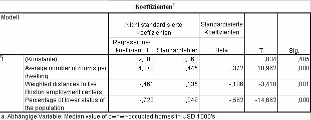
For the dependent variable mean house price in owner-occupied houses per district (in US $ 1000) from the Boston Housing data set, the regression model shown here is:
- Each additional room in the house increases the purchase price by US $ 4873,
- every additional kilometer to a workplace reduces the purchase price by US $ 461 and
- every percentage point more in the proportion of the lower-class population reduces the purchase price by US $ 723.
If you standardize all variables, you can estimate the influence of an explanatory variable on the dependent variable:
- The variable Proportion of the lower- class population has the greatest influence : −0.562,
- The second largest influence is the number of rooms : 0.372 and
- the variable distance to workplaces has the lowest influence: −0.106.
If the variables were independent of one another, one could use the squared regression coefficients to indicate the proportion of the explained variance:
- The variable proportion of the lower-class population explains almost 32% of the variance in the mean house price ( ),
- the variable number of rooms explains almost 14% of the variance in the mean house price ( ) and
- the variable distance to workplaces explains a little more than 1% of the variance in the mean house price ( ).


