Expected value

The expected value (seldom and ambiguous mean ), which is often abbreviated with, is a basic concept of stochastics . The expected value of a random variable describes the number that the random variable assumes on average. For example, if the underlying experiment is repeated indefinitely, it is the average of the results. The law of large numbers describes the exact form in which the averages of the results tend towards the expected value as the number of experiments increases, or, in other words, how the sample means converge towards the expected value as the sample size increases . ${\displaystyle \mu }$

It determines the localization (position) of the distribution of the random variables and is comparable to the empirical arithmetic mean of a frequency distribution in descriptive statistics. It is calculated as the probability-weighted mean of the values ​​that the random variable assumes. However, it does not have to be one of these values ​​itself. In particular, the expected value can assume the values . ${\displaystyle \pm \infty }$

Because the expected value only depends on the probability distribution , we speak of the expected value of a distribution without reference to a random variable. The expectation value of a random variable can be viewed as the center of gravity of the probability mass and is therefore referred to as its first moment .

motivation

The numbers on the dice can be viewed as different characteristics of a random variable . Because the (actually observed) relative frequencies, according to the law of large numbers, approach the theoretical probabilities of the individual numbers as the sample size increases , the mean value must strive towards the expected value of . To calculate it, the possible values ​​are weighted with their theoretical probability. ${\displaystyle X}$ ${\displaystyle n}$ ${\displaystyle X}$

${\displaystyle {\begin{array}{lcl}\operatorname {E} (X)&=&1\cdot P(X=1)+2\cdot P(X=2)+3\cdot P(X=3)+4\cdot P(X=4)+5\cdot P(X=5)+6\cdot P(X=6)\\&=&(1+2+3+4+5+6)\cdot {\tfrac {1}{6}}=3{,}5.\end{array}}}$

Like the results of the die rolls, the mean value is random . In contrast to this, the expected value is a fixed indicator of the distribution of the random variables . ${\displaystyle X}$

The definition of the expected value is analogous to the weighted mean of empirically observed numbers. For example, if a series of ten dice attempts returned the results 4, 2, 1, 3, 6, 3, 3, 1, 4, 5, the associated mean value can

${\displaystyle {\bar {x}}=(4+2+1+3+6+3+3+1+4+5)\cdot {\tfrac {1}{10}}=3{,}2}$

alternatively can be calculated by first summarizing the same values ​​and weighting them according to their relative frequency :

${\displaystyle {\bar {x}}={\tfrac {2}{10}}\cdot 1+{\tfrac {1}{10}}\cdot 2+{\tfrac {3}{10}}\cdot 3+{\tfrac {2}{10}}\cdot 4+{\tfrac {1}{10}}\cdot 5+{\tfrac {1}{10}}\cdot 6=3{,}2}$.

In general, the mean of the numbers in throws can be like ${\displaystyle n}$

${\displaystyle 1\cdot h_{n}(1)+2\cdot h_{n}(2)+3\cdot h_{n}(3)+4\cdot h_{n}(4)+5\cdot h_{n}(5)+6\cdot h_{n}(6),}$

write in which denotes the relative frequency of the number . ${\displaystyle h_{n}(k)}$ ${\displaystyle k}$

Concept and notation

The concept of the expected value goes back to Christiaan Huygens . In a treatise on games of chance from 1656, "Van rekeningh in spelen van geluck", Huygens describes the expected win of a game as "het is my soo veel weerdt". Frans van Schooten used the term expectatio in his translation of Huygens' text into Latin . Bernoulli adopted the term introduced by van Schooten in his Ars conjectandi in the form valor expectationis .

In the western world is used for the operator , especially in Anglophone literature . ${\displaystyle \operatorname {E} \left(X\right)}$ ${\displaystyle \operatorname {E} \left[X\right]}$

The term can be found in Russian-language literature . ${\displaystyle M(X)}$

The designation emphasizes the property as a first moment that is not dependent on chance. The Bra-Ket notation is used in physics . In particular, instead of writing for the expected value of a quantity . ${\displaystyle \mu _{X}}$ ${\displaystyle \langle X\rangle }$ ${\displaystyle \operatorname {E} (X)}$ ${\displaystyle X}$

Definitions

If a random variable is discrete or has a density , the following formulas exist for the expected value.

Expected value of a discrete real random variable

In the real discrete case, the expected value is calculated as the sum of the products of the probabilities of each possible result of the experiment and the “values” of these results.

If a real discrete random variable that accepts the values with the respective probabilities (with as a countable index set ), the expected value in the case of existence is calculated with: ${\displaystyle X}$ ${\displaystyle (x_{i})_{i\in I}}$ ${\displaystyle (p_{i})_{i\in I}}$ ${\displaystyle I}$ ${\displaystyle \operatorname {E} (X)}$

${\displaystyle \operatorname {E} (X)=\sum _{i\in I}x_{i}p_{i}=\sum _{i\in I}x_{i}P(X=x_{i})}$

It should be noted that nothing is said about the order of the summation (see summable family ).

Is , then has a finite expectation if and only if the convergence condition ${\displaystyle I=\mathbb {N} }$ ${\displaystyle X}$ ${\displaystyle \operatorname {E} (X)}$

${\displaystyle \lim _{a\rightarrow \infty }\sum _{i=1}^{a}|x_{i}|p_{i}=\sum _{i=1}^{\infty }|x_{i}|p_{i}<\infty }$is fulfilled, ie the series for the expected value is absolutely convergent .

The following property is often useful for nonnegative integer random variables

${\displaystyle \operatorname {E} (X)=\sum \limits _{i=1}^{\infty }P(X\geq i).}$

This property is proven in the section on the expectation of a non-negative random variable.

Expected value of a real random variable with a density function

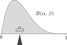
The expected value balances the probability mass - here the mass below the density of a beta (α, β) distribution with the expected value α / (α + β).

If a real random variable has a probability density function , i.e. if the image measure has this density with respect to the Lebesgue measure , then the expected value in the case of existence is calculated as ${\displaystyle X}$ ${\displaystyle f}$ ${\displaystyle P^{X}}$ ${\displaystyle \lambda }$

(1) ${\displaystyle \displaystyle \quad \operatorname {E} (X)=\int _{\mathbb {R} }xf(x)\,\mathrm {d} \lambda (x).}$

In many applications there is (generally improper ) Riemann integrability and the following applies:

(2) ${\displaystyle \displaystyle \quad \operatorname {E} (X)=\int _{-\infty }^{\infty }xf(x)\,\mathrm {d} x.}$

It is equivalent to this equation if the distribution function of is: ${\displaystyle F}$ ${\displaystyle X}$

(3) ${\displaystyle \displaystyle \quad \operatorname {E} (X)=\int _{0}^{\infty }(1-F(x))\,\mathrm {d} x-\int _{-\infty }^{0}F(x)\,\mathrm {d} x.}$

(2) and (3) are equivalent under the common assumption ( is a density function and is a distribution function of ), which can be proven with school-based means. ${\displaystyle f}$ ${\displaystyle F}$ ${\displaystyle X}$

For nonnegative random variables, the important relationship to the reliability function follows from this ${\displaystyle R(t)=1-F(t)}$

${\displaystyle \operatorname {E} (X)=\int _{0}^{\infty }(1-F(t))\,\mathrm {d} t=\int _{0}^{\infty }R(t)\,\mathrm {d} t.}$

general definition

The expected value is to correspond to the Lebesgue integral with respect to the probability measure defined: Is a measure of the relative integrated or quasi integrable random variable on a probability space with values in , wherein the Borel σ algebra over , it is defined as ${\displaystyle X}$ ${\displaystyle P}$ ${\displaystyle (\Omega ,\Sigma ,P)}$ ${\displaystyle ({\overline {\mathbb {R} }},{\mathcal {B}})}$ ${\displaystyle {\mathcal {B}}}$ ${\displaystyle {\overline {\mathbb {R} }}:=\mathbb {R} \cup \{-\infty ,\infty \}}$

${\displaystyle \operatorname {E} (X)=\int _{\Omega }X\,\mathrm {d} P=\int _{\Omega }X(\omega )\mathrm {d} P(\omega )\,}$.

The random variable has an expected value precisely when it is quasi-integrable , i.e. the integrals ${\displaystyle X}$

${\displaystyle \int _{\Omega }X^{+}(\omega )\,\mathrm {d} P(\omega )}$ and ${\displaystyle \int _{\Omega }X^{-}(\omega )\,\mathrm {d} P(\omega )}$

are not both infinite, where and denote the positive as well as the negative part of . In this case, or can apply. ${\displaystyle X^{+}}$ ${\displaystyle X^{-}}$ ${\displaystyle X}$ ${\displaystyle \operatorname {E} (X)=\infty }$ ${\displaystyle \operatorname {E} (X)=-\infty }$

The expectation value is finite if and only if it is integrable, i.e. the above integrals over and both are finite. This is equivalent to ${\displaystyle X}$ ${\displaystyle X^{+}}$ ${\displaystyle X^{-}}$

${\displaystyle \int _{\Omega }|X(\omega )|\,\mathrm {d} P(\omega )<\infty .}$

In this case, many authors write that the expected value exists or is a random variable with an existing expected value , and thus exclude the case or respectively . ${\displaystyle X}$ ${\displaystyle \infty }$ ${\displaystyle -\infty }$

Expected value of two random variables with a common density function

Have the integrable random variables and a joint probability density function , then the expectation value of a function calculated from and according to the set of Fubini to ${\displaystyle X}$ ${\displaystyle Y}$ ${\displaystyle f(x,y)}$ ${\displaystyle g(X,Y)}$ ${\displaystyle X}$ ${\displaystyle Y}$

${\displaystyle \operatorname {E} (g(X,Y))=\int _{-\infty }^{\infty }\int _{-\infty }^{\infty }g(x,y)f(x,y)\,\mathrm {d} x\,\mathrm {d} y}$

The expectation of is only finite if the integral ${\displaystyle g(X,Y)}$

${\displaystyle \int _{-\infty }^{\infty }\int _{-\infty }^{\infty }\left|g(x,y)\right|f(x,y)\,\mathrm {d} x\,\mathrm {d} y}$

is finite.

In particular:

${\displaystyle \operatorname {E} (X)=\int _{-\infty }^{\infty }\int _{-\infty }^{\infty }xf(x,y)\,\mathrm {d} x\,\mathrm {d} y}$

The expected value is calculated from the edge density as in the case of univariate distributions:

${\displaystyle \operatorname {E} (X)=\int _{-\infty }^{\infty }xf_{X}(x)\,\mathrm {d} x}$

The edge density is given by ${\displaystyle f_{X}(x)}$

${\displaystyle f_{X}(x)=\int _{-\infty }^{\infty }f(x,y)\,\mathrm {d} y}$

Elementary properties

Linearity

The expectation value is linear , so it holds for any, not necessarily independent random variable that ${\displaystyle X_{1},X_{2}}$

${\displaystyle \operatorname {E} (aX_{1}+bX_{2})=a\operatorname {E} (X_{1})+b\operatorname {E} (X_{2})}$

is. There are special cases

${\displaystyle \operatorname {E} (cX+d)=c\operatorname {E} (X)+d}$,

${\displaystyle \operatorname {E} (cX)=c\operatorname {E} (X)}$

and

${\displaystyle \operatorname {E} (d)=d}$.

The linearity can also be extended to finite sums:

${\displaystyle \operatorname {E} \left(\sum _{i=1}^{n}X_{i}\right)=\sum _{i=1}^{n}\operatorname {E} (X_{i})}$

The linearity of the expected value follows from the linearity of the integral.

monotony

Is almost certain , and there are so true ${\displaystyle X\leq Y}$ ${\displaystyle \operatorname {E} (X),\operatorname {E} (Y)}$

${\displaystyle \operatorname {E} (X)\leq \operatorname {E} (Y)}$.

Probabilities as expected values

The probabilities of events can also be expressed using the expected value. For every event applies ${\displaystyle A}$

${\displaystyle \operatorname {P} (A)=\operatorname {E} (\chi _{A})\,}$,

where is the indicator function of . ${\displaystyle \chi _{A}}$ ${\displaystyle A}$

This connection is often useful, for example to prove the Chebyshev inequality .

Triangle inequality

It applies

${\displaystyle \left|\operatorname {E} (X)\right|\leq \operatorname {E} (|X|)}$

and

${\displaystyle \operatorname {E} (|X+Y|)\leq \operatorname {E} (|X|)+\operatorname {E} (|Y|)}$

Examples

roll the dice

An illustration of the convergence of averages of rolling a dice to the expected value of 3.5 as the number of tries increases.

The experiment is a throw of the dice . We consider the number of points rolled as a random variable , with each of the numbers 1 to 6 being rolled with a probability of 1/6. ${\displaystyle X}$

${\displaystyle \operatorname {E} (X)=\sum _{i=1}^{6}i\cdot {\frac {1}{6}}=3{,}5}$

For example, if you roll the dice 1000 times, i.e. you repeat the random experiment 1000 times and add up the rolled numbers and divide by 1000, the result is with a high probability a value close to 3.5. However, it is impossible to get this value with a single roll of the dice.

Saint Petersburg Paradox

The Saint Petersburg Paradox describes a game of chance whose random win has an infinite expected value. According to classical decision theory, which is based on the expected value rule, one should risk an arbitrarily high stake. However, since the probability of losing the stake is 50%, this recommendation does not seem rational. One solution to the paradox is to use a logarithmic utility function . ${\displaystyle X}$ ${\displaystyle X\succcurlyeq Y\Leftrightarrow \operatorname {E} (X)\geq \operatorname {E} (Y)}$

Random variable with density

The real random variable is given with the density function ${\displaystyle X}$

${\displaystyle f(x)={\begin{cases}{\frac {1}{x}},&3\leq x\leq 3\mathrm {e} ,\\&\\0,&{\text{sonst}}\end{cases}}}$

where denotes Euler's constant. ${\displaystyle \mathrm {e} }$

The expected value of is calculated as ${\displaystyle X}$

${\displaystyle {\begin{aligned}\operatorname {E} (X)&=\int _{-\infty }^{\infty }xf(x)\,\mathrm {d} x=\int _{-\infty }^{3}x\cdot 0\,\mathrm {d} x+\int _{3}^{3\mathrm {e} }x\cdot {\frac {1}{x}}\,\mathrm {d} x+\int _{3\mathrm {e} }^{\infty }x\cdot 0\,\mathrm {d} x\\&=0+\int _{3}^{3\mathrm {e} }1\,\mathrm {d} x+0=[x]_{3}^{3\mathrm {e} }=3\mathrm {e} -3=3(\mathrm {e} -1).\end{aligned}}}$

general definition

Given is the probability space with , the power set of and for . The expected value of the random variable with and is ${\displaystyle (\Omega ,\Sigma ,P)}$ ${\displaystyle \Omega =\{\omega _{1},\omega _{2},\omega _{3}\}}$ ${\displaystyle \Sigma }$ ${\displaystyle \Omega }$ ${\displaystyle P(\{\omega _{i}\})={\tfrac {1}{3}}}$ ${\displaystyle i=1,2,3}$ ${\displaystyle X\colon \Omega \to \mathbb {R} }$ ${\displaystyle X(\omega _{1})=X(\omega _{2})=1}$ ${\displaystyle X(\omega _{3})=2}$

${\displaystyle \operatorname {E} (X)=\int _{\Omega }X\,\mathrm {d} P=X(\omega _{1})P(\{\omega _{1}\})+X(\omega _{2})P(\{\omega _{2}\})+X(\omega _{3})P(\{\omega _{3}\})=1\cdot {\frac {1}{3}}+1\cdot {\frac {1}{3}}+2\cdot {\frac {1}{3}}={\frac {4}{3}}}$

Since it is a discrete random variable with and , the expected value can alternatively be calculated as ${\displaystyle X}$ ${\displaystyle P(X=1)=P(\{\omega _{1},\omega _{2}\})={\tfrac {2}{3}}}$ ${\displaystyle P(X=2)=P(\{\omega _{3}\})={\tfrac {1}{3}}}$

${\displaystyle \operatorname {E} (X)=1\cdot P(X=1)+2\cdot P(X=2)=1\cdot {\frac {2}{3}}+2\cdot {\frac {1}{3}}={\frac {4}{3}}}$

Other properties

Expected value of a non-negative random variable

If is and is almost certainly non-negative, then according to Fubini-Tonelli's theorem (here the square brackets denote the predicate mapping ) ${\displaystyle p>0}$ ${\displaystyle X\in L^{p}}$

${\displaystyle \operatorname {E} (X^{p})=\int _{\Omega }X(\omega )^{p}\,\mathrm {d} P(\omega )=\int _{\Omega }\int _{0}^{\infty }px^{p-1}[x\leq X(\omega )]\,\mathrm {d} x\,\mathrm {d} P(\omega )=\int _{0}^{\infty }\int _{\Omega }px^{p-1}[x\leq X(\omega )]\,\mathrm {d} P(\omega )\,\mathrm {d} x=p\int _{0}^{\infty }x^{p-1}P{\big (}\{\omega \in \Omega \mid x\leq X(\omega ){\big )}\,\mathrm {d} x}$

So is

${\displaystyle \operatorname {E} (X^{p})=p\int _{0}^{\infty }x^{p-1}P(X\geq x)\,\mathrm {d} x=p\int _{0}^{\infty }x^{p-1}P(X>x)\,\mathrm {d} x.}$

(The last equality is correct, there for almost everyone .) ${\displaystyle P(X=x)=0}$ ${\displaystyle x\in \mathbb {R} }$

The following known special case results for: ${\displaystyle p=1}$

${\displaystyle \operatorname {E} (X)=\int _{0}^{\infty }P(X\geq x)\,\mathrm {d} x=\int _{0}^{\infty }P(X>x)\,\mathrm {d} x.}$

For integer, nonnegative random variables, the following applies because

${\displaystyle \int _{n}^{n+1}P(X>x)\,\mathrm {d} x=P(X\geq n+1)}$

the above formula:

${\displaystyle \operatorname {E} (X)=\sum _{i=0}^{\infty }\int _{i}^{i+1}P(X>x)\,\mathrm {d} x=\sum _{i=0}^{\infty }P(X\geq i+1)=\sum _{i=1}^{\infty }P(X\geq i).}$

Sigma additivity

If all random variables are almost certainly non-negative, the finite additivity can even be extended to -additivity: ${\displaystyle (X_{i})_{i\in \mathbb {N} }}$ ${\displaystyle \sigma }$

${\displaystyle \operatorname {E} \left(\sum _{i=1}^{\infty }X_{i}\right)=\sum _{i=1}^{\infty }\operatorname {E} (X_{i})}$

Expected value of the product of n stochastically independent random variables

If the random variables are stochastically independent of one another and can be integrated, the following applies: ${\displaystyle X_{i}}$

${\displaystyle \operatorname {E} \!\left(\prod _{i=1}^{n}X_{i}\right)=\prod _{i=1}^{n}\operatorname {E} (X_{i})}$

especially too

${\displaystyle \operatorname {E} \!\left(X_{i}X_{j}\right)=\operatorname {E} \!\left(X_{i}\right)\cdot \operatorname {E} \!\left(X_{j}\right)}$ For ${\displaystyle i\neq j}$

Expected value of the product of non-stochastically independent random variables

If the random variables are independent and not stochastically, the following applies to their product: ${\displaystyle X}$ ${\displaystyle Y}$

${\displaystyle \operatorname {E} \!\left(XY\right)=\operatorname {E} \!\left(X\right)\operatorname {E} \!\left(Y\right)+\operatorname {Cov} \!\left(X,Y\right)}$

It is the covariance between and . ${\displaystyle \operatorname {Cov} \!\left(X,Y\right)}$ ${\displaystyle X}$ ${\displaystyle Y}$

Expected value of a composite random variable

Is a composite random variable, say are independent random variables and are identically distributed and is on defined, it can be represented as ${\displaystyle Y}$ ${\displaystyle N,X_{1},X_{2},\dots }$ ${\displaystyle X_{i}}$ ${\displaystyle N}$ ${\displaystyle \mathbb {N} _{0}}$ ${\displaystyle Y}$

${\displaystyle Y:=\sum _{i=1}^{N}X_{i}}$.

If the first moments of exist , then applies ${\displaystyle N,X_{1},X_{2},\dots }$

${\displaystyle \operatorname {E} (Y)=\operatorname {E} (N)\operatorname {E} (X_{1})}$.

This statement is also known as the formula of Wald . She is z. B. used in insurance mathematics.

Monotonous convergence

If the non-negative random variables are almost certainly monotonically growing point by point and almost certainly converge to another random variable , then the following applies ${\displaystyle (X_{i})_{i\in \mathbb {N} }}$ ${\displaystyle X}$

${\displaystyle \lim _{i\to \infty }\operatorname {E} (X_{i})=\operatorname {E} (X)}$.

This is the theorem of monotonic convergence in the probabilistic formulation.

Calculation using the cumulant generating function

The cumulative generating function of a random variable is defined as

${\displaystyle g_{X}(t)=\ln \operatorname {E} (e^{tX})}$.

If it is derived and evaluated at 0, the expected value is:

${\displaystyle \operatorname {E} (X)=g'_{X}(0)}$.

The first cumulant is the expected value.

Calculation using the characteristic function

The characteristic function of a random variable is defined as . With their help, the expected value of the random variable can be determined by deriving: ${\displaystyle X}$ ${\displaystyle \varphi _{X}(t):=\operatorname {E} (e^{itX})}$

${\displaystyle \operatorname {E} (X)={\frac {\varphi _{X}'(0)}{\mathrm {i} }}}$.

Calculation using the torque generating function

Similar to the characteristic function, the torque generating function is defined as

${\displaystyle M_{X}(t):=\operatorname {E} \left(e^{tX}\right)}$.

Here, too, the expected value can easily be determined as

${\displaystyle \operatorname {E} (X)=M_{X}'(0)}$.

This follows from the fact that the expected value is the first moment and the k-th derivatives of the moment-generating function at 0 are exactly the k-th moments.

Calculation using the probability generating function

If only natural numbers are accepted as values, the expected value for can also be determined with the help of the probability-generating function ${\displaystyle X}$

${\displaystyle m_{X}(t):=\operatorname {E} \left(t^{X}\right)}$.

to calculate. It then applies

${\displaystyle \operatorname {E} \left[X\right]=\lim _{t\uparrow 1}m_{X}'(t)}$,

if the left-hand limit exists.

Best approximation

If a random variable is in a probability space , the best approximation describes an in the sense of minimizing , where a is a real constant. This follows from the best approximation theorem, da ${\displaystyle X}$ ${\displaystyle (\Omega ,\Sigma ,P)}$ ${\displaystyle \operatorname {E} \left(X\right)}$ ${\displaystyle X}$ ${\displaystyle \operatorname {E} \left(\left(X-a\right)^{2}\right)}$

${\displaystyle \langle X-\operatorname {E} (X),b\rangle =0}$

for all constants , where denotes the standard normal scalar product . This view of the expected value makes the definition of the variance as the minimum mean square distance meaningful, see also the Fréchet principle . ${\displaystyle b}$ ${\displaystyle \langle .,.\rangle }$ ${\displaystyle L^{2}}$

Expected values ​​of functions of random variables

If there is a random variable again, the expected value of can also be determined using the formula instead of using the definition: ${\displaystyle Y=g(X)}$ ${\displaystyle Y}$

${\displaystyle \operatorname {E} (Y)=\operatorname {E} (g(X))=\int _{-\infty }^{\infty }g(x)f_{X}(x)\,\mathrm {d} x}$

In this case, too, the expected value only exists if

${\displaystyle \int _{-\infty }^{\infty }\left|g(x)\right|f_{X}(x)\,\mathrm {d} x}$

converges.

For a discrete random variable, a sum is used:

${\displaystyle \operatorname {E} (Y)=\operatorname {E} (g(X))=\sum _{i}g(x_{i})p_{X}(x_{i}).}$

If the sum is not finite, then the series must converge absolutely in order for the expectation value to exist.

Related concepts and generalizations

Location parameters

→ Main article : measure of position (stochastics)

If the expected value is understood as the center of gravity of the distribution of a random variable, then it is a situation parameter. This indicates where the main part of the distribution is located. Further location parameters are

1. The mode : The mode indicates the point at which the distribution has a maximum, i.e. in the case of discrete random variables the characteristic with the greatest probability and in the case of continuous random variables the maximum positions of the density function. In contrast to the expected value, the mode always exists, but does not have to be unique. Examples of ambiguous modes are bimodal distributions .
2. The median is another common location parameter. It indicates which value on the x-axis separates the probability density in such a way that half of the probability is found to the left and right of the median. The median also always exists, but does not have to be unique (depending on the definition).

Moments

If the expected value is understood as the first moment , it is closely related to the higher-order moments. Since these are in turn defined by the expected value in connection with a function , they are, as it were, a special case. Some of the familiar moments are: ${\displaystyle g(\cdot )}$

• The variance : Centered second moment . Here is the expected value. ${\displaystyle g(X)=(X-\mu _{X})^{2}}$ ${\displaystyle \mu _{X}}$
• The skewness : centered third moment, normalized to the third power of the standard deviation . It is . ${\displaystyle \sigma _{X}}$ ${\displaystyle g(X)={\frac {(X-\mu _{X})^{3}}{\sigma _{X}^{3}}}}$
• The curvature : Centered fourth moment, normalized to . It is . ${\displaystyle \sigma _{X}^{4}}$ ${\displaystyle g(X)={\frac {(X-\mu _{X})^{4}}{\sigma _{X}^{4}}}}$

Conditional expected value

The conditional expected value is a generalization of the expected value for the case that certain outcomes of the random experiment are already known. This allows conditional probabilities to be generalized and the conditional variance to be defined. The conditional expectation value plays an important role in the theory of stochastic processes .

Quantum mechanical expectation

If the wave function of a particle is in a certain state and is an operator, then is ${\displaystyle \psi (r,t)=\langle r|\psi (t)\rangle }$ ${\displaystyle |\psi (t)\rangle }$ ${\displaystyle {\hat {O}}}$

${\displaystyle \langle {\hat {O}}\rangle _{|\psi (t)\rangle }:=\langle \psi (t)|{\hat {O}}|\psi (t)\rangle =\int _{M^{2}}\mathrm {d} ^{n}r\,\mathrm {d} ^{n}r^{\prime }\,\psi ^{\star }(r,t)\langle r|{\hat {O}}|r^{\prime }\rangle \psi (r^{\prime },t)}$

the quantum mechanical expectation of in the state . is here the spatial space in which the particle moves, is the dimension of , and a superscript star stands for complex conjugation . ${\displaystyle {\hat {O}}}$ ${\displaystyle |\psi (t)\rangle }$ ${\displaystyle M}$ ${\displaystyle n}$ ${\displaystyle M}$

If it can be written as a formal power series (and this is often the case), the formula is used ${\displaystyle {\hat {O}}}$ ${\displaystyle O({\hat {r}},{\hat {p}})}$

${\displaystyle \langle {\hat {O}}\rangle _{\psi }=\int _{M}\mathrm {d} ^{n}r\,\psi ^{\star }(r,t)O(r,{\frac {\hbar }{i}}\nabla _{r})\psi (r,t).}$

The index on the expectation value bracket is not only abbreviated as here, but sometimes also omitted entirely.

example

The expected value of the whereabouts in the location representation is

${\displaystyle \langle {\hat {r}}\rangle =\int _{M}\mathrm {d} ^{n}r\,\psi ^{\star }(r,t)r\psi (r,t)=\int _{M}\mathrm {d} ^{n}r\,r|\psi (r,t)|^{2}=\int _{M}\mathrm {d} ^{n}r\,rf(r,t).}$

The expected value of the location in the momentum representation is

${\displaystyle \langle {\hat {r}}\rangle =\int _{M}\mathrm {d} ^{n}p\,\Psi ^{\star }(p,t)i\hbar {\vec {\nabla }}_{p}\Psi (p,t),}$

where we have identified the probability density function of quantum mechanics in space.

Expected value of matrices and vectors

→ Main article : Covariance matrix

Let be a stochastic - matrix , with the stochastic variables as elements, then the expected value of is defined as: ${\displaystyle \mathbf {X} }$ ${\displaystyle m\times n}$ ${\displaystyle (X_{i,j})}$ ${\displaystyle \mathbf {X} }$

${\displaystyle \operatorname {E} \left(\mathbf {X} \right)=\operatorname {E} {\begin{pmatrix}X_{1,1}&X_{1,2}&\cdots &X_{1,n}\\X_{2,1}&X_{2,2}&\cdots &X_{2,n}\\\vdots &\vdots &\ddots &\vdots \\X_{m,1}&X_{m,2}&\cdots &X_{m,n}\end{pmatrix}}={\begin{pmatrix}\operatorname {E} (X_{1,1})&\operatorname {E} (X_{1,2})&\cdots &\operatorname {E} (X_{1,n})\\\operatorname {E} (X_{2,1})&\operatorname {E} (X_{2,2})&\cdots &\operatorname {E} (X_{2,n})\\\vdots &\vdots &\ddots &\vdots \\\operatorname {E} (X_{m,1})&\operatorname {E} (X_{m,2})&\cdots &\operatorname {E} (X_{m,n})\end{pmatrix}}}$.

If there is a - random vector : ${\displaystyle n\times 1}$ ${\displaystyle \mathbf {X} }$

${\displaystyle \operatorname {E} (\mathbf {X} )=\operatorname {E} {\begin{pmatrix}X_{1}\\X_{2}\\\vdots \\X_{n}\end{pmatrix}}={\begin{pmatrix}\operatorname {E} (X_{1})\\\operatorname {E} (X_{2})\\\vdots \\\operatorname {E} (X_{n})\end{pmatrix}}={\begin{pmatrix}\mu _{1}\\\mu _{2}\\\vdots \\\mu _{n}\end{pmatrix}}={\boldsymbol {\mu }}}$.

See also

• Expectation utility function
• Expected value rule

literature

• Krishna B. Athreya , Soumendra N. Lahiri : Measure Theory and Probability Theory (=  Springer Texts in Statistics ). Springer Verlag , New York 2006, ISBN 0-387-32903-X ( MR2247694 ).
• Heinz Bauer : Probability Theory (=  De Gruyter textbook ). 5th, revised and improved edition. de Gruyter , Berlin, New York 2002, ISBN 3-11-017236-4 ( MR1902050 ).
• Kai Lai Chung : A Course in Probability Theory . Academic Press, Inc. , San Diego (et al.) 2001, ISBN 0-12-174151-6 ( R1796326 ).
• Walter Greiner : Quantum Mechanics . 6. revised and exp. Edition. Publisher Harri Deutsch , Zurich [u. a.] 2005, ISBN 3-8171-1765-5 .
• Erich Härtter : Probability calculation for economists and natural scientists . 10th edition. Vandenhoeck & Ruprecht , Göttingen 1974, ISBN 3-525-03114-9 .
• Norbert Henze : Stochastics for beginners . 10th edition. Springer Spectrum , Wiesbaden 2013, ISBN 978-3-658-03076-6 , doi : 10.1007 / 978-3-658-03077-3 .
• Achim Klenke : Probability Theory . 3rd, revised and expanded edition. Springer Spectrum , Berlin, Heidelberg 2013, ISBN 978-3-642-36017-6 , doi : 10.1007 / 978-3-642-36018-6 .
• Norbert Kusolitsch : Measure and probability theory . An introduction (=  Springer textbook ). 2nd, revised and expanded edition. Springer-Verlag, Berlin, Heidelberg 2014, ISBN 978-3-642-45386-1 .
• M. Loève : Probability Theory I (=  Graduate Texts in Mathematics . Volume 45 ). 4th edition. Springer Verlag, Berlin, Heidelberg 1977, ISBN 3-540-90210-4 ( MR0651017 ).
• Vladimir Spokoiny , Thorsten Dickhaus : Basics of Modern Mathematical Statistics (=  Springer Texts in Statistics ). Springer-Verlag, Heidelberg, New York, Dordrecht, London 2015, ISBN 978-3-642-39908-4 ( MR3289985 ).

Web links

• Interactive visualization of cube example

Individual evidence

1. ↑ Norbert Henze: Stochastics for beginners . Vieweg + Teubner, 2008. ISBN 978-3-8348-9465-6 . P. 79.
2. ↑ See for example AN Širjaev: Probability 1988, p. 52 ff!
3. ^ John Aldrich: Earliest Uses of Symbols in Probability and Statistics . on-line
4. ↑ Ross, SM: Introduction to probability models , Academic Press, 2007, 9th edition, p. 143, ISBN 0-12-598062-0 .
5. ↑ H. Wirths: The expectation value - sketches for the development of concepts from grade 8 to 13. In: Mathematik in der Schule 1995 / Heft 6, pp. 330–343.