Bayesian game

A Bayesian game , Bayesian game , or Bayesian game , describes in game theory a game with incomplete information , which is named after the English mathematician Thomas Bayes . The Bayes' theorem , by which one conditional probabilities can be calculated, constitutes the basis for solutions of this variety.

Bayesian games can be modeled as games with imperfect information .

definition

In a game with incomplete information there is at least one player who does not have all the information about the other players that is decisive for the game (generally payout functions). Bayesian games cannot be analyzed a priori. Assumptions have to be made about the strategies and decisions of the other players in the form of probability distributions ( beliefs ).

According to a model by Harsanyi , Bayesian games are represented and analyzed as games with imperfect information with the help of such beliefs . In such a game there is at least one player who is not aware of every decision made previously (both other players and random decisions). For all random decisions not made by players, a new player ( called nature ) is introduced who makes them before all other decisions. The same solution concepts can thus be used as in games with imperfect information.

For example, in card games, the distribution of the cards is random and therefore unknown in most cases. Looking at the distribution of the cards as the first train of the player Nature , so players imperfect information about the decisions taken so far have. In contrast, chess is a classic example of games with perfect information.

Formally, the following applies to a game : ${\displaystyle G=<N;\;<T_{i};\;S_{i};\;u_{i};\;p_{i}>_{i\in N}>}$

1. N denotes the set of players
2. ${\displaystyle T_{i}}$denotes the possible types of player i. This is the type chosen by nature, are the types of all other players. ${\displaystyle t_{i}}$ ${\displaystyle t_{-i}}$
3. ${\displaystyle S_{i}}$is the set of all possible strategies of player i. This is a chosen strategy and are the strategies of all other players. ${\displaystyle s_{i}}$ ${\displaystyle s_{-i}}$
4. ${\displaystyle u_{i}(s_{i};\;s_{-i};\;t_{i};\;t_{-i})}$is the payout function for players i. This depends on all the strategies and types chosen.
5. ${\displaystyle p_{i}}$are the player's beliefs i.

A balance consists of each player's strategy and their beliefs . A strategy is a set of actions for every possible type.

Mathematical Foundations (Bayes' Theorem)

Graphical illustration of Bayes' theorem

→ Main article : Bayes' theorem

With the help of Bayes' theorem, conditional probabilities can be calculated:

${\displaystyle P(A_{i}|B)\;=\;{\frac {P(B|A_{i})\cdot P(A_{i})}{P(B)}}}$

The following applies to the probability of conditional : ${\displaystyle A_{i}}$ ${\displaystyle B}$

${\displaystyle {\begin{aligned}P(A_{i}|B)\;&=\;{\frac {P(A_{i}\cap B)}{P(B)}}\\&=\;{\frac {{\frac {P(A_{i}\cap B)}{P(A_{i})}}\cdot P(A_{i})}{P(B)}}\\&=\;{\frac {P(B|A_{i})\cdot P(A_{i})}{P(B)}}\end{aligned}}}$

Clearly therefore - as in the picture on the right - is the probability that arrives (red), with the knowledge that has been received (yellow area), just the portion of the over to leading branch at all to leading branches. ${\displaystyle A_{i}}$ ${\displaystyle B}$ ${\displaystyle A_{i}}$ ${\displaystyle B}$ ${\displaystyle B}$

Non-sequential games and sequential games

Sequential games are round-based games where the player payouts are just the sum of the player payouts in each round. If the strategy amounts and payout functions are identical in each round, one also speaks of repeated games . However, this is not a requirement for sequential games.

Different forms of representation are suitable depending on the type of game. Usually the normal form is only used for non-sequential games. The extensive form , on the other hand, is used for both non-sequential and sequential games.

Signal games denote a special type of sequential Bayesian games, which are usually represented in a variant of the extensive form.

Stochastic Bayesian games model sequential Bayesian games with environmental states and stochastic state transitions.

Non-sequential games

Bayesian Nash equilibrium

Example 1: non-sequential Bayesian game with player types

Bayesian Nash Equilibrium is a combination of strategies (if any) in which no player can improve their expected payout by changing strategies. He has to take into account his assumptions about the probability distribution ( beliefs ) for the strategies of the other players. This concept is analogous to the Nash equilibrium in the case of games with perfect and complete information.

example

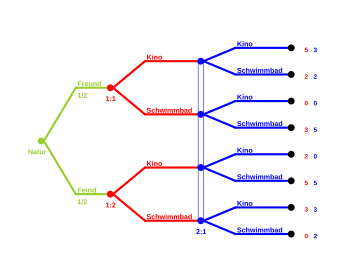
In this game, two work colleagues plan their leisure activities. There is a choice between a swimming pool and a cinema. Player 1 would rather go to the cinema, Player 2 would prefer the swimming pool. Of course, both of them prefer to spend their free time with a friend rather than an enemy. However, Player 2 doesn't know how much Player 1 likes him.

Player 1 is either friend or enemy type and he knows his type himself. The payouts depend on their relationship to each other and the choice of leisure activity: If they are friends and visit the same facility, they will receive a payout of 3. If they are enemies, they prefer to avoid each other and receive a payout of 3 if they are not at the same place Place are. In addition, they receive payment 2 for their preferred leisure activity.

The probability distribution of the types of player 1 is common knowledge and evenly distributed: . Since the players decide at the same time (no agreement possible), player 2 must make assumptions about the choice of player 1. ${\displaystyle P({\text{Freund}})=P({\text{Feind}})={\tfrac {1}{2}}}$

There are two Bayesian Nash equilibria in which no player can be better off by deviating from his strategy.

In the first equilibrium with ([cinema, swimming pool]; cinema), P (cinema | friend) = 1 and P (swimming pool | enemy) = 1. Thus, according to Bayes, it follows that P (friend | cinema) = P (enemy | swimming pool) = 1. An analogous procedure in the second equilibrium with ([swimming pool, cinema]; swimming pool) yields in total:

${\displaystyle {\begin{aligned}&([{\text{Kino}},{\text{Schwimmbad}};&{\text{Kino}})&;{\text{ mit }}P({\text{Freund}}|{\text{Kino}})=P({\text{Feind}}|{\text{Schwimmbad}})=1\;)\\&([{\text{Schwimmbad}},{\text{Kino}};&{\text{Schwimmbad}})&;{\text{ mit }}P({\text{Feind}}|{\text{Kino}})=P({\text{Freund}}|{\text{Schwimmbad}})=1\;)\\\end{aligned}}}$

Sequential games

Perfect Bayesian balance

→ Main article : Perfect Bayesian balance

The perfect Bayesian equilibrium is a further development of the subgame-perfect equilibrium for games with incomplete information.

A lot of strategies and assumptions about probability distributions ( beliefs ) are called perfect Bayesian equilibrium if the following conditions are met:

1. Each player must be able to specify beliefs for each information set, which assigns a probability to each node of this set.
2. Every player acts rationally , given his beliefs and the strategy of his opponents. That is, the strategies lead to subgame-perfect results.
3. The beliefs on the equilibrium path are determined with the help of Bayes' theorem.

Note: Strictly speaking, these requirements only define a weakly perfect Bayesian equilibrium. Another condition is required for a perfect Bayesian equilibrium.

Examples

example 1

Example 1: Beer Quiche Game

In the so-called beer quiche game (first treated by Cho and Kreps ) there are two players:

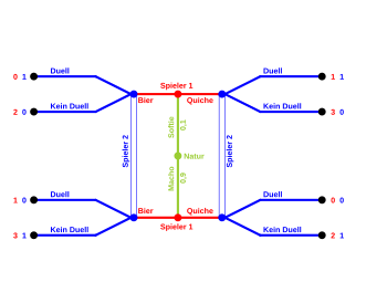
Player 1 is either a softie or a macho. The type of player 1 is determined by nature and is only known to him. Both players know the probability distribution: and . He has the choice of ordering beer or quiche for breakfast. As a softie he gets a payout of 1 from quiche and 0 from beer, and vice versa as a macho. ${\displaystyle P(Softie)=0,1}$ ${\displaystyle P(Macho)=0,9}$

Player 2 later meets player 1 and has the opportunity to duel. However, he only wants to duel if player 1 is a softie. However, player 2 does not know the type of player 1, only his breakfast order (signal). Player 1 does not want a duel under any circumstances and does not always get a payout for any duel 2. Player 2 receives payout 1 if he duels a softie or avoids a duel with a macho. In all other cases he receives a payout of 0.

The graphic on the right illustrates this signal game with an accumulated payout.

Possible strategies for player 1 are:

1. Play beer no matter if macho or softie, in short: [beer, beer],
2. Games Quiche whether macho or softy: [Quiche, Quiche]
3. Play beer as macho and quiche as softie: [beer, quiche] and
4. Games Quiche as macho and beer as a softie: [quiche, beer].

Possible strategies for player 2 are:

1. Always play a duel , regardless of the signal, in short: [duel, duel],
2. Always play no duel , regardless of the signal: [no duel, no duel],
3. Play a duel if there is a beer signal , otherwise no duel : [duel, no duel] and
4. Play No duel , if Signal Bier , otherwise duel : [No duel, duel].

There are two perfectly Bayesian equilibria:

In the first equilibrium with ([Quiche, Quiche]; [Duel, No Duel]), P (Quiche | Softie) = P (Quiche | Macho) = 1. With Bayes' theorem, according to requirement 3, the amount of the player results 2:

${\displaystyle P(Softie|Quiche)={\frac {P(Quiche|Softie)\cdot P(Softie)}{P(Quiche)}}={\frac {1\cdot 0,1}{1}}=0,1}$.

Similarly, in the second equilibrium ([beer, beer]; [no duel, duel]) the beliefs result . ${\displaystyle P(Softie|Bier)=0,1}$

So overall:

${\displaystyle {\begin{aligned}&((&[Quiche&,Quiche]&;\;[Duell,Kein\;Duell])&;\;P(Softie|Quiche)=0,1){\text{ und}}\\&((&[Bier&,Bier]&;\;[Kein\;Duell,Duell])&;\;P(Softie|Bier)=0,1)\end{aligned}}}$

Both equilibria meet the requirements for a perfect Bayesian equilibrium, but Cho and Kreps add another requirement to the concept of equilibrium. In general, this is called the intuitive criterion and ensures that the first equilibrium is ruled out.

Example 2

This example illustrates how beliefs are adjusted over the course of a repeated game using Bayes' theorem. There is only one player who bets on the outcome of any manipulated coin toss. A correct forecast pays 1, otherwise 0. The possible coin types are given by nature and are equally likely: Always heads (IK) , fair coins (FM) and always tails (IZ) .

In the first round, the player sets his beliefs according to the probability distribution of the types on (1/3; 1/3; 1/3) for (IK; FM; IZ). First, Strategy Head brings the same expected payout as Strategy Tails . The player can bet on heads or tails and then flips the coin. Before he bets again, he adjusts his beliefs using Bayes' theorem:

Head ( K ) is thrown:

Change in beliefs depending on the event

${\displaystyle {\begin{aligned}P(IK|K)&={\frac {P(K|IK)\cdot P(IK)}{P(K)}}&&={\frac {1\cdot 1/3}{1/2}}&&={\frac {2}{3}}\\P(FM|K)&={\frac {P(K|FM)\cdot P(FM)}{P(K)}}&&={\frac {1/2\cdot 1/3}{1/2}}&&={\frac {1}{3}}\\P(IZ|K)&={\frac {P(K|IZ)\cdot P(IZ)}{P(K)}}&&={\frac {0\cdot 1/3}{1/2}}&&=0\\\end{aligned}}}$

Number ( Z ) is thrown:

${\displaystyle {\begin{aligned}P(IK|Z)&={\frac {P(Z|IK)\cdot P(IK)}{P(Z)}}&&={\frac {0\cdot 1/3}{1/2}}&&=0\\P(FM|Z)&={\frac {P(Z|FM)\cdot P(FM)}{P(Z)}}&&={\frac {1/2\cdot 1/3}{1/2}}&&={\frac {1}{3}}\\P(IZ|Z)&={\frac {P(Z|IZ)\cdot P(IZ)}{P(Z)}}&&={\frac {1\cdot 1/3}{1/2}}&&={\frac {2}{3}}\\\end{aligned}}}$

If the game continues, the beliefs are adjusted as above. It is only to note that the probabilities or change after each throw. Assuming that the head fell in the first throw , the following applies: ${\displaystyle P(K)}$ ${\displaystyle P(Z)}$

${\displaystyle {\begin{aligned}P(K)&=P(IK|K)\cdot P(IK)+P(FM|K)\cdot P(FM)+P(IZ|K)\cdot P(IZ)={\tfrac {2}{3}}\cdot 1+{\tfrac {1}{3}}\cdot {\tfrac {1}{2}}+0\cdot 0={\tfrac {5}{6}}{\text{ und}}\\P(Z)&=1-P(K)={\tfrac {1}{6}}\end{aligned}}}$

Overall, on the first move, the player bets randomly ( equally distributed ) on heads or tails . Then he will continue to bet on the result of the first round until the opposite occurs. If this case occurs at all, he will choose his strategy again at random from this point in time, since it is certainly a fair coin.

See also

• Game theory
• Nash equilibrium
• Partial perfect balance
• Signal game

literature

• Robert Gibbons: A Primer in Game Theory . Financial Times, Harlow 1992, ISBN 978-0-7450-1159-2 .
• Drew Fudenberg, Jean Tirole: Game Theory . The MIT Press, Cambridge, Massachusetts 1991, ISBN 978-0-262-06141-4 .
• John A. Hartigan: Bayes Theory . Springer, New York, Heidelberg 1983, ISBN 3-540-90883-8 .

Individual evidence

1. ^ John C. Harsanyi: Games with Incomplete Information Played by "Bayesian" Players Part I. The Basic Model . In: Management Science . tape 14 , no. 3 , 1967, p. 127-261 , doi : 10.1287 / mnsc.14.3.159 , JSTOR : 30046151 .
2. ^ Drew Fudenberg, Jean Tirole: Game Theory . The MIT Press, Cambridge, Massachusetts 1991, ISBN 978-0-262-06141-4 . P. 209 ff.
3. ^ Stefano Albrecht, Jacob Crandall, and Subramanian Ramamoorthy. Belief and Truth in Hypothesized Behaviors. Artificial Intelligence, 235, 2016, pp. 63-94, doi: 10.1016 / j.artint.2016.02.004
4. ^ In-Koo Cho and David M. Kreps: Signaling Games and Stable Equilibria . In: The Quarterly Journal of Economics . tape 102 , no. 2 , 1987, pp. 183-187 , JSTOR : 1885060 .
5. ^ In-Koo Cho and David M. Kreps: Signaling Games and Stable Equilibria . In: The Quarterly Journal of Economics . tape 102 , no. 2 , 1987, pp. 185 , JSTOR : 1885060 .