Axonometry

• 

  Axonometry of a house on squared paper

• 

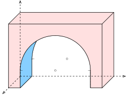
  Archway (circles) in cavalier projection

The axonometry is a method in the descriptive geometry to relatively simple three-dimensional objects in a plane display.

The coordinates of essential points and the images of the three coordinate axes in a drawing plane are used here. The result is a parallel projection for every choice of image axes except for a scaling . In general, the result is an oblique (or oblique) parallel projection. An orthogonal (or perpendicular) parallel projection is only obtained with a special choice of the image axes and the distortion ratios, i.e. the imaging rays are perpendicular to the image plane (see orthogonal axonometry ).

Principle of axonometry

Principle of axonometry

One imagines the coordinate axes together with the points projected onto a drawing plane with the help of parallel rays. The unit routes are usually reproduced in a distorted manner. The distortion ratios are denoted by , and . A point is now entered in the image with the coordinate axes as follows: ${\displaystyle (1,0,0),(0,1,0),(0,0,1)}$ ${\displaystyle v_{x}}$ ${\displaystyle v_{y}}$ ${\displaystyle v_{z}}$ ${\displaystyle P=(x,y,z)}$

You go from zero ${\displaystyle {\overline {O}}}$

to go in -direction, then ${\displaystyle x\cdot v_{x}}$ ${\displaystyle {\overline {x}}}$

around in -direction and eventually ${\displaystyle y\cdot v_{y}}$ ${\displaystyle {\overline {y}}}$

around in -direction. ${\displaystyle z\cdot v_{z}}$ ${\displaystyle {\overline {z}}}$

(The order can be reversed as desired.)

Since it is very laborious to construct the image axes and the distortions for a specific projection direction and position of the image plane, one simply selects the images of the coordinate axes in the drawing plane and specifies suitable distortions. The mathematical justification for this is Pohlke's theorem : For (almost) every choice of image axes and distortions, except for similarity (scaling), the image of a parallel projection is obtained. (The images of the coordinate axes must not fall on a straight line, the distortions should be greater than zero.)

Image axes and distortions

(For specifications in the area of technical drawing : see DIN 5 part 10.)

various distortions of a unit cube
(image plane parallel to the yz plane)

Parameters of special axonometries (the military projection is a bird's eye view)

Parameters of a general axonometry

The image impression is only good with a suitable choice of image axes and distortions. A good image effect is achieved if the image axes and the distortion ratios are chosen so that the result is a perpendicular parallel projection. Since you want to work with the simplest possible distortion ratios (e.g. 1 or 0.5), you can use the following examples (see illustration) as a guide when choosing the image axes and distortions. If you have square paper available, the following choice is available for axes and distortions: Two coordinate axes coincide with the main directions of the square paper, the third axis runs in the direction of the square diagonals (see opening picture). In order to keep the construction simple, you should choose the units on the horizontal and vertical axis two boxes and on the diagonal direction a box diagonal as the unit. This then results in the following distortions: equal to ≈ 0.7: 1: 1. ${\displaystyle v_{x}:v_{y}:v_{z}=1/{\sqrt {2}}:1:1}$

Axonometries with two equal distortions are called dimetric , with three equal distortions isometric , otherwise trimetric .

Definition:

• ${\displaystyle \alpha :}$Angle between the -axis and the -axis ${\displaystyle {\overline {z}}}$ ${\displaystyle {\overline {x}}}$
• ${\displaystyle \beta :}$Angle between the -axis and the -axis ${\displaystyle {\overline {z}}}$ ${\displaystyle {\overline {y}}}$
• ${\displaystyle \gamma :}$Angle between the -axis and the -axis ${\displaystyle {\overline {x}}}$ ${\displaystyle {\overline {y}}}$

Cavalier projection, cabinet projection

• Image plane parallel to the yz plane , d. H.
  • ${\displaystyle \beta =90^{\circ }}$ and
  • ${\displaystyle v_{y}=v_{z}=1}$.
• Note: In the literature, the terms cavalier perspective and cabinet perspective are not uniformly defined. The above definition is the most general. Further restrictions are often required:
  • Cabinet projection : additional and (dimetry), ${\displaystyle \alpha =\gamma =135^{\circ }}$ ${\displaystyle v_{x}=0.5}$
  • Cavalier projection: in addition and (isometry). ${\displaystyle \alpha =\gamma =135^{\circ }}$ ${\displaystyle v_{x}=1}$

Bird's eye view, military projection

• Image plane parallel to the xy plane , d. H.
  • ${\displaystyle \gamma =90^{\circ }}$ and
  • ${\displaystyle v_{x}=v_{y}=1}$ (Dimetry).
• The following also applies to the military projection: (Isometry). ${\displaystyle v_{z}=1}$

Such axonometries are used in city plans in order to achieve scale (horizontal) and clarity of buildings.

Engineer axonometry

In an engineering axonometry according to ISO 5456-3, the distortions are:

${\displaystyle {\begin{aligned}v_{x}&=0.5\\v_{y}=v_{z}&=1\end{aligned}}}$ (dimetric axonometry)

The axes are aligned as follows:

${\displaystyle {\begin{aligned}\alpha =\gamma &=132^{\circ }\\\beta &=97^{\circ }\end{aligned}}}$ (or 7 ° and 42 ° to the horizontal)

Set square with markings for engineering axonometry

Advantages of engineering axonometry are:

• simple distortions,
• almost vertical axonometry (good image effect, the scaling factor is 1.06),
• the outline of a sphere is a circle (otherwise it is an ellipse).

Math background

→ Main article : Orthogonal axonometry # Possible shortenings

An engineering axonometry corresponds to a perpendicular parallel projection onto a plane with the normal vector (= negative projection direction) with subsequent scaling by the factor . The plan of the normal vector forms an angle of with the x-axis . The angle with respect to the xy plane is . The exact angles between the images of the coordinate axes are: ${\displaystyle ({\sqrt {7}},1{,}1)^{\top }}$ ${\displaystyle {\tfrac {3}{2{\sqrt {2}}}}\approx 1{,}061}$ ${\displaystyle \arccos({\tfrac {\sqrt {7}}{2{\sqrt {2}}}})\approx 20{,}70^{\circ }}$ ${\displaystyle \arccos({\tfrac {2{\sqrt {2}}}{3}})\approx 19{,}47^{\circ }}$

• ${\displaystyle {\begin{aligned}\alpha &=\arccos(-{\tfrac {\sqrt {7}}{4}})&\approx 131{,}4^{\circ }\approx 2{,}294\\\beta &=\arccos(-{\tfrac {1}{8}})&\approx 97{,}18^{\circ }\approx 1{,}696\end{aligned}}}$

For the (dimetric) vertical parallel projection with (without scaling!) The following applies: ${\displaystyle v_{y}=v_{z}=2v_{x}}$

• ${\displaystyle {\begin{aligned}v_{x}&={\tfrac {\sqrt {2}}{3}}&\approx 0{,}471\\v_{y}=v_{z}&={\tfrac {2{\sqrt {2}}}{3}}&\approx 0{,}942\end{aligned}}}$.

Isometric axonometry

Examples in standard isometry: cube, cuboid, house and sphere

(Note the multiple meanings of the term isometry in mathematics.)

In isometric axonometry , or isometry for short , the distortions are all the same. The angles between the axis images can still be freely selected.

The following applies to the representation referred to as standard isometry :

• ${\displaystyle v_{x}=v_{y}=v_{z}=1}$ (all axes undistorted)
• ${\displaystyle \alpha =\beta =\gamma =120^{\circ }}$, where the axis is perpendicular ${\displaystyle {\overline {z}}}$

The advantages of this choice of parameters are:

• The coordinates can be adopted unchanged,
• The axonometric image is an orthogonal projection scaled by the factor (perpendicular parallel projection ). This results in a good picture effect and the outline of a sphere is a circle. ${\displaystyle {\sqrt {1.5}}=1.225}$
• Sign systems such as B. xfig , offer a triangular grid to facilitate the drawing of objects with axes parallel to the axis.

The "disadvantages" are:

• A blemish due to the symmetry is that two of the 8 corner points of an axially parallel cube coincide (see picture).

different axonometries of a tower

Overview of the special axonometries

With general axonometry, the two angles between the axes and the distortions can be chosen (almost) freely. So that all three axis images do not lie on a straight line, must be. This restriction for the choice of angles guarantees a view from above at an angle . The restriction provides views from below at an angle . It swaps the usual orientation from the x-axis to the y-axis. Negative distortions would change the usual orientation of the axes. ${\displaystyle 0<\alpha ,\beta }$ ${\displaystyle 0<v_{x},v_{y},v_{z}}$ ${\displaystyle 0<\alpha +\beta <360^{\circ }}$ ${\displaystyle 360<\alpha +\beta <720^{\circ }}$

Circles in axonometry

Axonometry: circles in cavalier projection

→ Main article : Ellipse (descriptive geometry)

With parallel projection, circles are generally mapped onto ellipses. An important special case: a circle whose circular plane is parallel to the picture board is shown undistorted. This is the case, for example, with a cavalier projection in which the yz plane (see example) is mapped without distortion. With a bird's eye view , all horizontal circles remain undistorted. If a circle is distorted into an ellipse (see picture), you can map some points and a tangent square and fit an ellipse into the picture of the square (parallelogram) by hand or with a drawing program. It should be noted that the images of perpendicular circular diameters are generally not the main axes of the image ellipse, but rather conjugate diameters . The main axes can be reconstructed from these with the help of the Rytz axis construction . The ellipse can then be drawn precisely with a drawing program or an elliptical compass. If you only have a pair of compasses, a ruler and a curved ruler at hand, the ellipse can be approximated surprisingly well and quickly with the help of the vertex circles of curvature (see Ellipse or C. Leopold, p. 64). In orthogonal axonometry you can usually get by without the complex Rytz construction.

Spheres in axonometry

Bird's eye view of a sphere with vz = 1

→ Main article : Sphere (descriptive geometry)

The outline of a sphere is simply a circle with the radius of the sphere only in orthogonal axonometry. Since both engineering axonometry and standard isometry are scaled orthogonal projections (see above), the outline of a sphere also appears here as a circle, albeit scaled. In any axonometric view, the outline of a sphere appears as an ellipse, which may irritate the viewer (see sphere in isometric bird's eye view). Therefore, scenes with spheres should better be mapped with orthogonal axonometry or at least with engineering axonometry or standard isometry.

swell

• Ulrich Graf, Martin Barner: Descriptive Geometry. Quelle & Meyer, Heidelberg 1961, ISBN 3-494-00488-9 .
• Fucke, Kirch, Nickel: Descriptive Geometry. Fachbuch-Verlag, Leipzig, 1998, ISBN 3-446-00778-4
• Cornelie Leopold: Geometric Basics of Architectural Representation. Verlag W. Kohlhammer, Stuttgart, 2005, ISBN 3-17-018489-X

Web links

Wiktionary: axonometry  - explanations of meanings, word origins, synonyms, translations

• Normal (orthogonal) axonometry with simple examples
• Descriptive geometry for architects (PDF; 1.5 MB). Script (Uni Darmstadt)
• Fundamentals and elements of traffic engineering ( Memento from August 10, 2013 in the Internet Archive ) (PDF; 493 kB) TU Dresden

Individual evidence

1. ↑ Hans Hoischen: Technical Drawing. Basics, standards, examples, descriptive geometry . 21st edition. Girardet, Düsseldorf 1986, ISBN 3-7736-2023-3 , p. 252 , 7.6.2 Dimetric projection DIN 5 part 2 .