Confidence interval for the probability of success of the binomial distribution

A confidence interval for the probability of success of the binomial distribution is a confidence interval (confidence interval ) for the parameter of the binomial distribution (after observing hits in a sample of the size ). ${\displaystyle p}$ ${\displaystyle k}$ ${\displaystyle n}$

Comparison of the methods discussed in this article to determine confidence intervals for the parameter of the binomial distribution (the confidence level here is equal to 0.95). ${\displaystyle p}$ ${\displaystyle \gamma }$

Exact confidence intervals, such as the Clopper-Pearson interval, can be obtained with the help of the binomial distribution . However, there are also approximation methods that (mostly) are based on the approximation of the binomial distribution by the normal distribution .

Introductory example

In order to estimate the unknown relative share of a political party A in the electorate, people are asked in an opinion poll whether they will vote for party A. The exact procedure is: We select a random person from the electorate 400 times and interview them. We do not record whether this person has already been interviewed. So it can happen, although even with a large electorate, it is unlikely that the same person will be questioned more than once. The number of respondents who say they vote for party A depends on chance and is therefore a random variable. Since the interviewed persons are selected randomly and independently of one another, the random variable is binomially distributed with the parameters and the unknown parameter . Let us assume that respondents in the survey indicated that they vote for party A. One calculates an estimate of as: ${\displaystyle p}$ ${\displaystyle n=400}$ ${\displaystyle X}$ ${\displaystyle X}$ ${\displaystyle n=400}$ ${\displaystyle p}$ ${\displaystyle k=20}$ ${\displaystyle {\hat {p}}}$ ${\displaystyle p}$

${\displaystyle {\hat {p}}={k \over n}=0{,}05\,}$.

This is called a point estimate because only one value is calculated as an estimate of . ${\displaystyle p}$

The true value of the relative fraction can be either less than or greater than the point estimate . The only thing that is certain is that any value between 0 and 1 can take on. A confidence interval for . If the procedure is repeated many times, the calculated confidence intervals should contain the parameter in "most cases" . How often this should be the case is expressed using the confidence level (or also the confidence level ) . The calculated interval is called the confidence interval (or confidence interval ). 95% is often chosen straight away. This means that if the procedure is repeated, the statement is correct for 95% of all samples . ${\displaystyle p}$ ${\displaystyle {\hat {p}}}$ ${\displaystyle p}$ ${\displaystyle [p_{u},p_{o}]}$ ${\displaystyle p}$ ${\displaystyle p}$ ${\displaystyle \gamma }$ ${\displaystyle [p_{u},p_{o}]}$ ${\displaystyle \gamma }$ ${\displaystyle p\in [p_{u},p_{o}]}$

Simple approximation through the normal distribution

Coverage probability of the standard interval for n = 400.

The following simple approximation formula is often used:

${\displaystyle c=\Phi ^{-1}\left(1-{\alpha \over 2}\right)}$, where the level of error and the quantile function of the standard normal distribution, i.e. the inverse function of its distribution function. ${\displaystyle \alpha =1-\gamma }$ ${\displaystyle \Phi ^{-1}}$ ${\displaystyle \Phi }$

${\displaystyle p_{u}={\hat {p}}-c\cdot {\sqrt {{\hat {p}}\cdot (1-{\hat {p}}) \over n}}\,}$

${\displaystyle p_{o}={\hat {p}}+c\cdot {\sqrt {{\hat {p}}\cdot (1-{\hat {p}}) \over n}}}$,

which is also called the standard interval .

If this formula is used, should and be. However, using the standard interval can be problematic. The figure shows the coverage probability for and as an example . It is often below the required level of 0.95. ${\displaystyle k\geq 50}$ ${\displaystyle n-k\geq 50}$ ${\displaystyle n=400}$ ${\displaystyle p\in [0{,}125;0{,}875]}$

Clopper-Pearson interval

C. Clopper and Egon Pearson (1934) gave the following exact procedure to determine the lower limit and the upper limit . As before, let the size of the sample, the number of successes and the confidence level be 95%. ${\displaystyle p_{u}}$ ${\displaystyle p_{o}}$ ${\displaystyle n}$ ${\displaystyle k}$

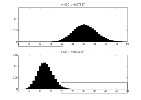
The upper limit is determined from and the lower limit from , see figure. The lower limit can not be specified with this formula. ${\displaystyle P(X\leq k;p_{o})=0{,}025}$ ${\displaystyle P(X\geq k;p_{u})=0{,}025}$ ${\displaystyle k=0}$

Explanation: If the probability of achieving maximum success for a unit value falls below the limit 0.025, then with a maximum error probability of 2.5% it can be excluded that the unit value is sought. Thus, p _{o is} the largest value of at which, given the confidence level, it can still be assumed that k or fewer successes will occur. This seems too improbable for larger values ​​of . ${\displaystyle k}$ ${\displaystyle p}$ ${\displaystyle p}$ ${\displaystyle p}$ ${\displaystyle p}$

For the lower limit, the following applies accordingly: is the smallest value of at which it is still assumed that or more successes can occur. For smaller values ​​of , this seems too improbable, although the probability of error here is a maximum of 2.5%. Thus, the statement “ and ” is correct in at least 95% of all cases . ${\displaystyle p_{u}}$ ${\displaystyle p}$ ${\displaystyle k}$ ${\displaystyle p}$ ${\displaystyle p\leq p_{o}}$ ${\displaystyle p\geq p_{u}}$

Practical calculation

The two values ​​p _u , p _o can be z. B. Calculate with the Excel function BETAINV. The function returns the quantile of the specified beta distribution back and is obtained due to the relationship of the binomial and beta distribution for the resolution of the equation : . In the following, as before, we denote the confidence level with , and is . ${\displaystyle P_{p}(X\leq k)=\alpha }$
${\displaystyle p=\operatorname {BETAINV} (1-\alpha ;k+1;n-k)}$ ${\displaystyle \gamma }$ ${\displaystyle \alpha =1-\gamma }$

In the example with a confidence level of 95%, the following is obtained for the lower limit of the confidence interval: P (X ≥ 20) = 0.025 P (X ≤ 19) = 0.975 ${\displaystyle n=400,k=20}$


${\displaystyle p_{u}=\operatorname {BETAINV} (1-0{,}975;20;400-19)=0{,}03081}$

and for the upper limit of the confidence interval:
${\displaystyle P(X\leq 20)=0{,}025}$
${\displaystyle p_{o}=\operatorname {BETAINV} (1-0{,}025;21;400-20)=0{,}07617}$

Explanation in words: Even with a vote share of only 3.1%, the probability that there are at least 20 people in the sample is still 2.5%. And accordingly: even with a vote share of 7.6%, the probability that there are at most 20 people in the sample is still 2.5%

The method is summarized in the following table:

	general case	Special case
lower limit	p u = BETAINV (α / 2; k; n-k + 1)	p u = 0 for k = 0
upper limit	p o = BETAINV (1-α / 2; k + 1; nk)	p o = 1 for k = n

Analysis of the coverage probability

If the confidence interval is successful, then according to the definition one demands that for all the coverage probability greater than or equal ; is. In the case of continuous distributions, confidence intervals can be found so that equality exists here (i.e. instead of ). This is not possible for the discrete binomial distribution. The following figure shows the coverage probability as a function of . Incidentally, the Clopper-Pearson interval is called exact because it ensures a coverage probability that is actually greater than or equal to the required confidence level for all . This is not the case for the approximations discussed below: Here there are often coverage probabilities that are smaller than the required level! ${\displaystyle C(k)}$ ${\displaystyle k}$ ${\displaystyle p}$ ${\displaystyle P_{p}(k\in \{0,\ldots ,n\}:p\in C(k))}$ ${\displaystyle \gamma }$ ${\displaystyle =\gamma }$ ${\displaystyle \geq \gamma }$ ${\displaystyle p}$ ${\displaystyle p}$

The coverage probability is calculated depending on and as follows: ${\displaystyle p}$ ${\displaystyle n}$

${\displaystyle P_{p}(k\in \{0,\ldots ,n\}:p\in C(k))=\sum _{k=0}^{n}B(k|p,n)\cdot \mathbf {1} _{[p_{u}(k),p_{o}(k)]}(p)}$.

Here is the indicator function . It assumes the value 1 if it is in the confidence interval, and otherwise the value 0. One sets for and one sets for . ${\displaystyle \mathbf {1} _{[p_{u}(k),p_{o}(k)]}(p)}$ ${\displaystyle p}$ ${\displaystyle k=0}$ ${\displaystyle p_{u}=0}$ ${\displaystyle k=n}$ ${\displaystyle p_{o}=1}$

Coverage probability of the Clopper-Pearson interval for and . It is above the required confidence level for everyone . ${\displaystyle n=40}$ ${\displaystyle n=400}$ ${\displaystyle p}$

Wilson interval

For n = 1, ..., 40, the coverage probability for the Clopper-Pearson interval is plotted here. It is always greater than γ = 0.95.

With the standard interval, the coverage probability for n = 1, ..., 40 is almost always below the required confidence level.

The coverage probability for the Wilson interval for n = 1, ..., 40.

The coverage probability for the Agresti-Coull interval for n = 1, ..., 40.

This interval was proposed by Edwin Bidwell Wilson in 1927 and is more accurate than the simple approximation by the normal distribution. The same applies as in the section on the approximation by the normal distribution , ${\displaystyle c}$

${\displaystyle p_{o,u}={\frac {1}{1+{\frac {c^{2}}{n}}}}\cdot \left({\hat {p}}+{\frac {c^{2}}{2n}}\pm c\cdot {\sqrt {{\frac {{\hat {p}}\cdot (1-{\hat {p}})}{n}}+{\frac {c^{2}}{4n^{2}}}}}\,\right)}$

Obviously the interval limits for large converge to the limits of the standard interval (since and with increasing go to zero). ${\displaystyle n}$ ${\displaystyle c^{2}/2n}$ ${\displaystyle c^{2}/4n^{2}}$ ${\displaystyle n}$

Forming gives the formula (4) given by Brown / Cai / DasGupta on page 107:

${\displaystyle p_{o,u}={\frac {k+{\frac {c^{2}}{2}}}{n+c^{2}}}\pm {\frac {c{\sqrt {n}}}{n+c^{2}}}\cdot {\sqrt {{\frac {k}{n}}\left(1-{\frac {k}{n}}\right)+{\frac {c^{2}}{4n}}}}}$

The figure shows the coverage probability for . ${\displaystyle n=1,\ldots ,40}$

The formula given by Henze on page 228 differs from this by a continuity correction (of +0.5 or −0.5 applied to ). ${\displaystyle k}$

Agresti-Coull interval

For that interval are employed , , and uses the (above-described) simple approximation with these parameters: ${\displaystyle {\tilde {k}}=k+{\frac {c^{2}}{2}}}$ ${\displaystyle \,{\tilde {n}}=n+c^{2}}$ ${\displaystyle \,{\tilde {p}}={\frac {\tilde {k}}{\tilde {n}}}}$

${\displaystyle p_{o,u}={\tilde {p}}\pm c\cdot {\sqrt {{\tilde {p}}\cdot (1-{\tilde {p}}) \over {\tilde {n}}}}}$

The midpoint of the interval is identical to that of the Wilson interval and the interval is never shorter than a Wilson interval.

If γ = 0.95, then and you get a simple rule: , and . ${\displaystyle c=1{,}96\approx 2}$ ${\displaystyle {\tilde {k}}=k+2}$ ${\displaystyle {\tilde {n}}=n+4}$ ${\displaystyle {\tilde {p}}={\frac {k+2}{n+4}}}$

Discussion of the advantages and disadvantages of the procedures

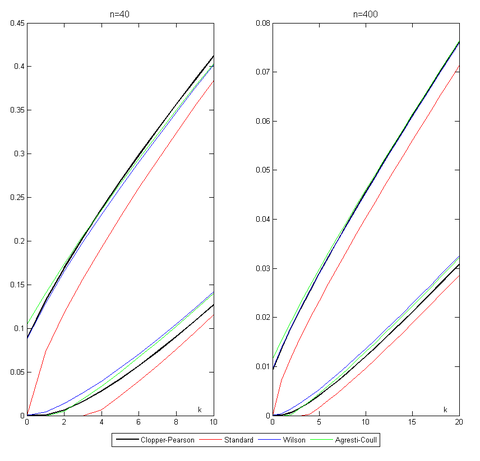
The methods described are compared in the basic article by Brown / Cai / DasGupta. There the standard interval is also called the Wald interval (after Abraham Wald ). Brown / Cai / DasGupta recommend three interval methods: the Wilson interval, the Agresti-Coull interval, and the Jeffreys interval, which we have not discussed here. For a graphical comparison of the upper and lower limits for the four methods, see the illustration at the beginning of this page.

literature

• Alan Agresti, Brent A. Coull: Approximate is better than 'exact' for interval estimation of binomial proportions. In: The American Statistician. 52, 1998, pp. 119-126. doi: 10.1080 / 00031305.1998.10480550 JSTOR 2685469
• Lawrence D. Brown, T. Tony Cai, Anirban DasGupta: Interval Estimation for a Binomial Proportion. In: Statistical Science. 16 (2), 2001, pp. 101-133. doi: 10.1214 / ss / 1009213286 JSTOR 2676784
• C. Clopper, ES Pearson : The use of confidence or fiducial limits illustrated in the case of the binomial. In: Biometrika. 26, 1934, pp. 404-413. doi: 10.1093 / biomet / 4/26/404 JSTOR 2331986
• TD Ross: Accurate confidence intervals for binomial proportion and Poisson rate estimation. In: Computers in Biology and Medicine. 33, 2003, pp. 509-531. doi: 10.1016 / S0010-4825 (03) 00019-2
• EB Wilson : Probable inference, the law of succession, and statistical inference. In: Journal of the American Statistical Association. 22, 1927, pp. 209-212. doi: 10.1080 / 01621459.1927.10502953 JSTOR 2276774
• Norbert Henze : Stochastics for Beginners: An Introduction to the Fascinating World of Chance. 8th edition. Vieweg + Teubner Verlag, 2010, ISBN 978-3-8348-0815-8 , doi: 10.1007 / 978-3-8348-9351-2 .
• Ulrich Krengel: Introduction to probability theory and statistics. 8th edition. Vieweg, 2005.
• Horst Rinne: Pocket book of statistics. Harri Deutsch, 2003.

Web links

• Be careful with the sigma rule from: Praxis der Mathematik, Heft 67 (2016) pp. 44–47

Individual evidence

1. ↑ The main methods are compared in the basic article by Brown / Cai / DasGupta. In addition to those specified here, z. B. discussed the Jeffreys interval.
2. ↑ See for this and also for the Clopper-Pearson and Wilson intervals, page 459 of the pocket book of statistics by Horst Rinne.
3. ↑ See Krengel, Chapter 4.7, section Confidence Intervals for the Probability of Success
4. ↑ See Brown / Cai / DasGupta, p. 108
5. ↑ Your article is supplemented by five comments from (1) Alan Agresti and Brent A. Coull (2) George Casella (3) Chris Corcoran and Cyrus Mehta (4) Malay Ghosh (5) Thomas J. Santner and concluded with a reply from Brown / Cai / DasGupta.