
LV PIPE II
LV PIPE II is the name of a software for a stress calculation program for spatial piping systems. The integration in Excel makes it easy to use and flexible. It enables a quick and extensive analysis of piping systems of any geometric configuration and complexity.
Program features
The LV PIPE II program determines u. a. the following sizes:
- Support forces and moments
- Expansion joints
- Pipe forces and moments
- Nozzle load
- Shifts
- Wind loads
- Tensions
- friction
- Spring hanger data
- Camp with play
Data are determined for the pure weight load case (assembly), the pure temperature load case (start-up / shutdown) and for the combined load case (operation). The most important parameters can be displayed graphically for easier assessment.
history
In a certain sense, piping technology has always been the pioneer in the use of computer programs. This applies to the area of isometric drawing using CAD programs as well as to the area of material management with material extracts and pipe spec management. This early appearance of EDP was particularly pronounced in the field of hydraulics and stress analysis.
The necessity of calculating the expansion of spatial pipeline systems and thus achieving a certain level of operational reliability was recognized early on. An ASCE article on this problem appeared as early as 1910. But was a spatial framework z. B. has been calculable for bridge constructions for a long time, an implementation of these calculation methods on a corresponding pipe framework failed due to the special features of the pipe bends. The movements that a loaded pipeline system makes in space were not understood for a long time. It was not until the pioneering work of Karman in 1911 and of Wahl and Hovgaard in 1928 that the way was paved for the calculation of three-dimensional piping systems with pipe bends.
With the knowledge gained, it was now possible to calculate simple frame structures such as expansion loops, L-legs and spatial Z-profiles. The expansion problem of complex line structures was reduced to the consideration of these known elementary frame structures. This procedure is still used today for a rough estimate of the flexibility or for the first creation of the support concept. Nevertheless, the growing risk potential in the chemical and petrochemical industry, but above all the problems in power plant technology, required a calculation of the entire pipeline system, including the consideration of singular supports, spring hangers and fixed point displacements. Out of this necessity, the Kellogg Company developed a general analytical method for calculating spatial piping systems in cooperation with various American universities in the 1930s . These procedures were refined over the years and officially published in 1941.
It was also the Kellogg Company that considered the use of digital computers to calculate spatial piping systems and had the first programs available on punch cards as early as 1954 . The profitability of these programs quickly became apparent. While the time required with these punch card programs had already shrunk to a tenth compared to manual calculations, the use of magnetic data carriers from 1956 reduced the calculation time again. The expansion of these programs was pushed further. The demands made on the programmers of the Kellogg Company in the early 1960s seem almost modern.
“Every conceivable pipeline configuration must be calculable, regardless of the number of branches, the fixed points, the supports and the internal ring connections. Above all, however, the program has to manage with minimal input effort and at the same time provide a maximum of automatisms. "
Why were such demands made of a pipe program in the early days of computer science ? With the help of the program, the calculator was freed from pure mathematical activity, but now had to describe the pipeline system to the program in an understandable manner. Furthermore, the calculator cannot decide whether it exceeds the possible complexity of a system that can just be calculated. The piping program must therefore be able to process every possible configuration and it must communicate with the user in a suitable manner.
It is obvious that a pipeline system with all its diversity and possible variations cannot be described as a whole. The practicable solution can only consist in reducing the whole problem to small, simple sub-problems. The fineness of the reduction is determined by the fixed pipe elements. It is therefore only necessary to describe the type, number, position and order of these finite elements in the program. The calculation method of the finite elements ( FEM ) had been researched mathematically, the problem could be solved via IT!
The various pipeline programs that emerged in Germany in the following years always followed this principle. The user first defines a Cartesian coordinate system in order to be able to describe points in space with a corresponding position vector. Then the given pipe system is divided into individual elements. These individual elements are distinguished from one another by the definition of connection nodes. A line element therefore always lies between two nodes. Conversely, this means that between two nodes, all properties such as diameter, wall thickness, material, but also the course of the line are constant. A line characteristic can only change at one node, and forces can only be introduced or removed and there can be supports at defined nodes. The position of all nodes in space is defined by a vector , which also defines the position of all elements. The load that occurs on a pipeline in operation is also not calculated as a whole, but is at least divided into the two basic load cases dead weight and temperature.
The programs themselves now process these finite elements according to the known mathematical methods. As a result of the calculation, the displacements, the forces and moments and the existing stresses are determined for each element and for each load case and documented accordingly.
How is the semantic description of a line system carried out? The programmer defines a set of keywords with which the user can determine the type of the individual elements, or with which the special properties of the elements and nodes can be defined. The programmer also defines a grammar that defines the position and order of the keywords in a data record.
These keywords and the associated grammar must be learned by the user. This common language learned enables the user to communicate with the program, i.e. to describe his problem to the program. The program itself now understands the problem, can process it and generate appropriate results.
Picture gallery

Logo created with LV PIPE II

Representation of the line nodes in LV PIPE II
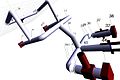
Exaggeratedly large line nodes and supports in LV PIPE II
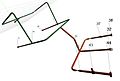
Color-coded representation of the stresses in a pipeline system with LV PIPE II

Representation of a deformed pipeline system with LV PIPE II


literature
- H.-J. Behrens (ed.): Pipeline technology. Compilation and editing B. Thier. 7th edition. Vulkan, Essen 1998, ISBN 3-8027-2713-4 , page 24ff.
Web links
Individual evidence
- ^ The MW Kellogg Company: Design of Piping Systems. Pullman Power Products, New York 1976