RANSAC algorithm

RANSAC ( English ran dom sa mple c onsensus , German as "match with a random sample") is a re-sampling - the algorithm for the estimation of a model within a series of measurements with outliers and coarse errors . Because of its robustness against outliers, it is primarily used in the evaluation of automatic measurements in the computer vision field. Here RANSAC supports - by calculating a data set adjusted for outliers, the so-called consensus set - compensation methods such as the method of least squares , which usually fail with a large number of outliers.

RANSAC was officially introduced in 1981 by Martin A. Fischler and Robert C. Bolles in the Communications of the ACM . An internal presentation at SRI International , on which both authors were working, took place in March 1980. M-estimators are an alternative to RANSAC . Compared to other estimators, such as the maximum likelihood estimators, these are more robust against outliers.

Introduction and principle

Often the result of a measurement is data points that represent physical values ​​such as pressure, distance or temperature, economic parameters or the like. A parameter-dependent model curve that fits as precisely as possible should be placed in these points. There are more data points available than are necessary to determine the parameters; the model is therefore overdetermined . The measured values ​​can contain outliers, i.e. values ​​that do not fit into the expected series of measurements . Since measurements were mostly carried out manually until the development of digital technology, the control by the surgeon meant that the proportion of outliers was usually low. The compensation algorithms used at that time , such as the least squares method, are well suited for the evaluation of such data sets with few outliers: With their help, the model is first determined with the entirety of the data points and then an attempt is made to detect the outliers.

The single outlier pulls the best-fit line upwards

With the development of digital technology from the beginning of the 1980s, the fundamentals changed. Due to the new possibilities, automatic measuring methods were increasingly used, especially in the field of computer vision . The result here is often a large number of values, which usually contain many outliers. The traditional methods assume a normal distribution of errors and sometimes do not provide a meaningful result if the data points contain many outliers. This is illustrated in the illustration opposite. A straight line (the model) is to be adapted to the points (measured values). On the one hand, the individual outliers among the 20 data points cannot be ruled out using traditional methods prior to determining the straight line. On the other hand, due to its position, it has a disproportionately strong influence on the regression line (so-called leverage point).

The RANSAC algorithm follows a new, iterative approach. Instead of equalizing all measured values ​​together, only as many randomly selected values ​​are used as are necessary to calculate the model parameters (in the case of a straight line, this would be two points). It is initially assumed that the selected values ​​are not outliers. This assumption is checked by first calculating the model from the randomly selected values ​​and then determining the distance of all measured values ​​(i.e. not only those originally selected) to this model. If the distance between a measured value and the model is less than a previously defined threshold value, then this measured value is not a gross error in relation to the calculated model. So he supports it. The more measured values ​​support the model, the more likely the values ​​randomly selected for the model calculation did not contain any outliers. These three steps - random selection of measured values, calculation of the model parameters and determination of the support - are repeated several times independently of one another. In each iteration, it is saved which measured values ​​support the respective model. This set is called the consensus set . From the largest consensus set , which ideally no longer contains any outliers, the solution is then determined using one of the traditional adjustment methods.

Applications

As mentioned, many outliers mainly occur with automatic measurements. These are often carried out in the computer vision field , so that RANSAC is particularly widespread here. Some applications are presented below.

Stitched panorama image of Alcatraz : To do this, individual images must be appropriately superimposed so that they can then be blended. To do this, common features must be found in the drawing files.

In image processing , RANSAC is used to determine homologous points between two camera images. The two image points that a single object point generates in the two images are homologous. The assignment of homologous points is called the correspondence problem. The result of an automatic analysis usually contains a large number of incorrect assignments. Procedures based on the result of the correspondence analysis use RANSAC to rule out incorrect assignments. An example of this approach is the creation of a panorama image from various smaller individual images ( stitching ). Another is the calculation of the epipolar geometry . This is a model from geometry that shows the geometric relationships between different camera images of the same object. Here RANSAC is used to determine the fundamental matrix, which describes the geometric relationship between the images.

In the DARPA Grand Challenge , a competition for autonomous land vehicles, RANSAC was used to determine the road surface and to reconstruct the movement of the vehicle.

The algorithm is also used to adapt geometrical bodies such as cylinders or the like in noisy three-dimensional point sets or to automatically segment point clouds . All points that do not belong to the same segment are regarded as outliers. After estimating the most dominant body in the point cloud, all points belonging to this body are removed so that further bodies can be determined in the next step. This process is repeated until all bodies in the point set have been found.

Procedure and parameters

The prerequisite for RANSAC is that more data points are available than are necessary to determine the model parameters. The algorithm consists of the following steps:

1. Randomly choose as many points from the data points as are necessary to calculate the parameters of the model. This is done in the expectation that this set will be free of outliers.
2. Determine the model parameters with the selected points.
3. Determine the subset of the measured values ​​whose distance from the model curve is smaller than a certain limit value (this subset is called the consensus set ). If it contains a certain minimum number of values, a good model has probably been found and the consensus set is saved.
4. Repeat steps 1-3 several times.

After performing several iterations, that subset is selected which contains the most points (if one was found). The model parameters are calculated using one of the usual compensation methods only with this subset. An alternative variant of the algorithm ends the iterations prematurely if enough points support the model in step 3. This variant is called preemptive - that is, prematurely terminating - RANSAC. With this approach, it must be known in advance how large the outlier portion is, so that it can be assessed whether sufficient measured values ​​support the model.

The algorithm essentially depends on three parameters:

1. the maximum distance of a data point from the model up to which a point is not considered a gross error;
2. the number of iterations and
3. the minimum size of the consensus set , i.e. the minimum number of points consistent with the model.

Maximum distance of a data point from the model

This parameter is fundamental to the success of the algorithm. In contrast to the other two parameters, it must be specified (the consensus set does not need to be checked , and the number of iterations can be selected to be almost unlimited). If the value is too large or too small, the algorithm can fail. This is illustrated in the following three pictures. One iteration step is shown in each case. The two randomly selected points with which the green model line was calculated are colored blue. The error bounds are shown as black lines. A point must lie within these lines to support the model line. If the distance chosen is too large, too many outliers will not be recognized, so that an incorrect model can have the same number of outliers as a correct model (Fig. 1a and 1b). If it is set too low, it can happen that a model that was calculated from an outlier-free set of values ​​is supported by too few other values ​​that are not outliers (Fig. 2).

• Problems if the choice of the error limit is too large or too small
• 

  1a. Correct solution, two points are outliers.

• 

  1b. Second, wrong solution with the same number of outliers as in 1a.

• 

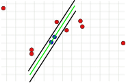
  2. Error bound too small.

Despite these problems, this value usually has to be determined empirically . The error limit can only be calculated using the laws of probability distribution if the standard deviation of the measured values ​​is known .

Number of iterations

The number of repetitions can be set in such a way that, with a certain probability, an outlier-free subset is selected from the data points at least once. If the number of data points that are necessary to calculate a model and the relative proportion of outliers in the data, then the probability is that at least one outlier is selected each time in the case of repetitions ${\displaystyle p}$ ${\displaystyle s}$ ${\displaystyle \epsilon }$ ${\displaystyle n}$

${\displaystyle p=1-\left(1-\left(1-\epsilon \right)^{s}\right)^{n}}$,

and so that this is at most , the choice must be large enough. Be at least more precise ${\displaystyle 1-p}$ ${\displaystyle n}$

${\displaystyle n={\frac {\log \left(1-p\right)}{\log \left(1-\left(1-\epsilon \right)^{s}\right)}}}$

Repetitions needed. The number therefore only depends on the proportion of outliers, the number of parameters of the model function and the specified probability of drawing at least one outlier-free subset. It is independent of the total number of measured values.

The table below shows the required number of repetitions depending on the outlier proportion and the number of points required to determine the model parameters. The probability of selecting at least one outlier-free subset from all data points is set at 99%.

Number of iterations required ( ) ${\displaystyle p=99\,\%}$

example	Number of points required	Outlier percentage
		10%	20%	30%	40%	50%	60%	70%
Straight	2	3	5	7th	11	17th	27	49
level	3	4th	7th	11	19th	35	70	169
Fundamental matrix	8th	9	26th	78	272	1177	7025	70188

Consensus set size

In the general variant of the algorithm, this value does not necessarily have to be known, since if a plausibility check is dispensed with, the largest consensus set can simply be used in the further course. However, knowledge of this is necessary for the variant that terminates prematurely. With this, the minimum size of the consensus set is usually determined analytically or experimentally. A good approximation is the total amount of measured values ​​minus the proportion of outliers that are suspected in the data. The minimum size is the same for data points . For example, with 12 data points and 20% outliers, the minimum size is approximately 10. ${\displaystyle \epsilon }$ ${\displaystyle n}$ ${\displaystyle (1-\epsilon )\cdot n}$

Adaptive determination of the parameters

The proportion of outliers in the total amount of data points is often unknown. It is therefore not possible to determine the required number of iterations and the minimum size of a consensus set . In this case, the algorithm is initialized with the worst-case assumption of an outlier proportion of 50%, for example, and the number of iterations and the size of the consensus set are calculated accordingly. After each iteration, the two values ​​are adjusted if a larger consistent set is found. If, for example, the algorithm is started with an outlier proportion of 50% and the calculated consensus set contains 80% of all data points, the result is an improved value for the outlier proportion of 20%. The number of iterations and the necessary size of the consensus set are then recalculated.

example

A straight line is to be fitted to a set of points in the plane. The points are shown in the first picture. The second picture shows the result of different runs. Red points support the straight line. Points whose distance from the straight line is greater than the error limit are colored blue. The third picture shows the solution found after 1000 iteration steps.

• RANSAC for adapting a straight line to data points
• 

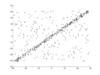
  1. Original data set.

• 

  2. Animation of several iterations.

• 

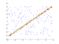
  3. Result after 1000 iterations.

Further developments

There are some extensions of RANSAC, two important ones of which are presented here.

LO-RANSAC

Model straight is not supported by all faultless points.

Experiments have shown that mostly more iteration steps than the theoretically sufficient number are necessary: ​​If a model is calculated with an outlier-free set of points, not all other values ​​that are not outliers have to support this model. The problem is illustrated in the figure opposite. Although the straight line was calculated using two error-free values ​​(black points), some other obviously correct points are classified as outliers (blue stars) in the top right of the image.

For this reason, the original algorithm for LO-RANSAC (locally optimized RANSAC) is expanded in step 3. As usual, the subset of the points that are not outliers is determined first. Then the model is determined again using this set and with the aid of any compensation method such as the least squares method. Finally, the subset is calculated whose distance to this optimized model is smaller than the error limit. Only this improved subset is saved as a consensus set .

MSAC

RANSAC selects the model that is supported by most of the measured values. This corresponds to the minimization of a sum in which all error-free values ​​are entered with 0 and all outliers with a constant value: ${\displaystyle C}$

${\displaystyle C=\sum _{i}p({\text{Fehler}})\quad {\text{mit}}\quad p=\left\{{\begin{array}{ll}0,&{\text{wenn Fehler}}<{\text{Fehlerschranke}}\\{\text{konstant}}&{\text{wenn Fehler}}\geq {\text{Fehlerschranke}}\end{array}}\right.}$

The calculated model can be very inaccurate if the error bound is set too high - the higher it is, the more solutions have the same values ​​for . In the extreme case, all errors in the measured values ​​are smaller than the error limit, so that it is always 0. This means that no outliers can be identified and RANSAC provides a poor estimate. ${\displaystyle C}$ ${\displaystyle C}$

MSAC ( M -Estimator SA mple C onsensus) is an extension of RANSAC that uses a modified objective function to be minimized:

${\displaystyle C=\sum _{i}p({\text{Fehler}})\quad {\text{mit}}\quad p=\left\{{\begin{array}{ll}{\text{Fehler,}}&{\text{wenn Fehler}}<{\text{Fehlerschranke}}\\{\text{konstanter Wert groesser als Fehlerschranke,}}&{\text{wenn Fehler}}\geq {\text{Fehlerschranke}}\end{array}}\right.}$

With this function, outliers continue to receive a certain “penalty” that is greater than the error threshold. Values ​​below the error limit are included in the total with the error instead of 0. This eliminates the problem mentioned, since a point contributes less to the total the better it fits the model.

Individual evidence

1. ^ Robert C. Bolles: Homepage at the SRI . ( online [accessed March 11, 2008]).
2. ↑ Martin A. Fischler: Homepage at SRI . ( online [accessed March 11, 2008]).
3. ↑ Martin A. Fischler and Robert C. Bolles: Random Sample Consensus: A Paradigm for Model Fitting with Applications to Image Analysis and Automated Cartography . March 1980 ( online (PDF; 301 kB) [accessed on September 13, 2007]).
4. ↑ Dag Ewering: Model-based tracking using line and point correlations . September 2006 ( online (PDF; 9.5 MB) [accessed on August 2, 2007]).
5. ^ Martin A. Fischler and Robert C. Bolles: RANSAC: An Historical Perspective . June 6, 2006 ( online ( MS PowerPoint ; 2.8 MB) [accessed March 11, 2008]).
6. ↑ Christian Beder and Wolfgang Förstner : Direct determination of cylinders from 3D points without using surface normals . 2006 ( uni-bonn.de [PDF; accessed on August 25, 2016]).
7. ^ Ondřej Chum, Jiři Matas and Štěpàn Obdržàlek: Enhancing RANSAC By Generalized Model Optimization . 2004 ( online [PDF; accessed August 7, 2007]).
8. ↑ PHS Torr and A. Zisserman: MLESAC: A new robust estimator with application to estimating image geometry . 1996 ( online (PDF; 855 kB) [accessed on August 7, 2007]).

literature

• Martin A. Fischler and Robert C. Bolles: Random Sample Consensus: A Paradigm for Model Fitting with Applications to Image Analysis and Automated Cartography. (PDF; 1.2 MB) 1981, accessed on October 14, 2019 . 
• Various authors: 25 Years of RANSAC, Workshop in conjunction with CVPR 2006. 2006, accessed March 11, 2008 . 
• Peter Kovesi: RANSAC - Robustly fits a model to data with the RANSAC algorithm (Matlab implementation). 2007, accessed March 11, 2008 . 
• Volker Rodehorst: Photogrammetric 3D reconstruction at close range through auto-calibration with projective geometry . wvb Wissenschaftlicher Verlag Berlin, 2004, ISBN 978-3-936846-83-6 (university publication, plus dissertation, TU Berlin 2004).
• Richard Hartley, Andrew Zisserman: Multiple View Geometry in Computer Vision . 2nd Edition. Cambridge University Press, Cambridge, UK 2004, ISBN 978-0-521-54051-3 (English).
• Tilo Strutz: Data Fitting and Uncertainty (A practical introduction to weighted least squares and beyond) . 2nd ed.Springer Vieweg, 2016, ISBN 978-3-658-11455-8 (English).

This article was added to the list of excellent articles on April 3, 2008 in this version .