Epipolar geometry

Two cameras record a scene from different points of view. The epipolar geometry describes the relationship between the two images.

The epipolar geometry (rarely also nuclear ray geometry ) is a mathematical model from geometry that represents the geometric relationships between different camera images of the same object. With their help, the dependency between corresponding image points can be described - i.e. the points that a single object point generates in the two camera images. Although its foundations were examined by Guido Hauck in 1883 , by Sebastian Finsterwalder in 1899 and by Horst von Sanden in 1908 , epipolar geometry only became more important with the automatic evaluation of digital images, especially in the field of machine vision .

The epipolar geometry is primarily used to obtain 3D information from images. It supports the correspondence analysis , i.e. the assignment of corresponding points, and considerably reduces the search effort required.

principle

Illustration with the pinhole camera

A camera can be geometrically modeled using a pinhole camera . In this, each point of the recorded object, the projection center and the associated image point lie on a straight line during the recording . If the object point was recorded twice from different positions, the intersection of the two straight lines and thus the coordinates of the object point can be calculated in a later evaluation using the orientations of the cameras. A 3D reconstruction is thus possible if the image points of an object point have been localized in both images. The epipolar geometry serves to support this localization: if the point is given in the first image, the search area in the second image is limited to a line if the epipolar geometry is known.

Schematic representation of the epipolar geometry

The geometric relationships are illustrated in the graphic on the left. In addition to the image and object points and the two projection centers, the two image planes of the two cameras are shown. These are folded in front of the projection centers. This makes the representation easier, but does not change the geometric relationships. The object point X is mapped onto the image point x _L in the camera image 1 . Starting from this image point, it is only possible to determine the associated ray on which X lies. Possible object points X ₁ , X ₂ or X ₃ , which, like X, correspond to the image point x _L , lie on this ray. This beam and thus all possible object points are imaged on a straight line when the object is recorded from a different position in the second image. The search for the image point x _R corresponding to the image point x _L in the second image is reduced to this .

With the help of the epipolar geometry, a simple relationship between corresponding points can be established without knowledge of the camera positions. Although information about the relative position of the cameras to one another can be derived from a known epipolar geometry, it is not necessary to know the camera positions explicitly to determine it. The epipolar geometry depends only on the parameters of the cameras and is therefore independent of the structure of the recorded scene.

Terms of epipolar geometry

Fixed terminology exists to describe epipolar geometry and its elements . The plane that spans the two projection centers of the cameras and the recorded object point is called the epipolar plane . This intersects the two images in a straight line, the so-called epipolar line . Only on this one can a corresponding pixel to a given point in the other image lie. The straight line that connects the two projection centers of the cameras penetrates the two image planes at one point, the epipole. The two epipoles do not change their position in the respective image as long as the position of the cameras to one another remains stable. The epipole of an image is also the image of the projection center of the other camera. All the epipolar lines of an image run through it, but depending on the position of the cameras in relation to one another, it can be outside the actual image.

In the field of photogrammetry, the terms nuclear beam geometry, core point, core plane and core line were and are still used in part instead of epipolar geometry, epipole, epipolar plane and epipolar line.

Applications

The epipolar geometry is mainly used in projective geometry , photogrammetry and computer vision . Its main purpose is to support correspondence analysis. If the corresponding point is sought in the other image for a prominent point in one image, the entire image must be examined if the epipolar geometry is unknown. If the epipolar geometry is known, the search for the corresponding point can be restricted to the epipolar line. This results in a considerable reduction in the search area . For this reason, epipolar geometry is primarily used where a scene or an object has to be analyzed quickly and with little effort in three dimensions using cameras. Important areas of application are computer-based vision , the measurement of workpieces for quality control, building surveys for architectural photogrammetry or aerial photogrammetry for creating maps .

Computer vision

When searching for correspondence for object identification, the epipolar geometry restricts the search area to the epipolar lines and thereby achieves an enormous saving in computing time. At the same time, by restricting the search area, it reduces the number of incorrect assignments of corresponding points. Both are of great advantage because they accelerate the algorithms and make them more reliable (more robust). In autonomous robotics in particular , simple calculations for short computing times are required, on the one hand because of the limited hardware on mobile platforms and on the other hand because of the need for quick reactions to avoid collisions. One participant in the DARPA Grand Challenge , a competition for unmanned land vehicles, used the OpenCV program library , which contains fast routines for calculating the epipolar geometry and its application in correspondence analysis.

Self-calibration of cameras

The 3D reconstruction of a scene from photographs requires that the internal and relative orientation of the cameras is known. Since the epipolar geometry describes the linear projective relationship between two images, it is used in the so-called self-calibration, i.e. the automatic determination of the camera parameters. The epipolar geometry is used to determine the (linear) inner orientation and the relative orientation from known correspondences (see section #Calculation ). Any existing (non-linear) distortion must have been determined beforehand by means of a camera calibration.

history

Fig. 1a from Table I in Hauck's article illustrates the quote.

The history of epipolar geometry is closely related to the history of photogrammetry . The first to analyze the underlying geometric relationships was the mathematician Guido Hauck. In 1883 he published an article in the Journal for Pure and Applied Mathematics in which the term core point was used for the first time :

"Let there be (Fig. 1a) and two projection levels, and the associated projection centers. We call the intersection of the two projection planes the basic section . Let the connecting line intersect the two projection planes at points and , which we call the core points of the two planes. " ${\displaystyle S'}$ ${\displaystyle S''}$ ${\displaystyle O_{1}}$ ${\displaystyle O_{2}}$ ${\displaystyle g_{12}}$ ${\displaystyle O_{1}O_{2}}$ ${\displaystyle o_{2}^{'}}$ ${\displaystyle o_{1}^{''}}$

- Guido Hauck : New Construction of Perspective and Photogrammetry . Journal for pure and applied mathematics, Volume 95, 1883, pages 1-35.

Based on the work of Hauck, Sebastian Finsterwalder developed an algorithm for a 3D reconstruction from two uncalibrated photos in 1899. Horst von Sanden wrote a first, more extensive presentation in 1908 as part of his dissertation The determination of the key points in photogrammetry . In this work he described methods for a simpler and more precise determination of the key points.

In the so-called analog photogrammetry with opto-mechanical photography and evaluation, which prevailed until the introduction of digital technology, the correspondence analysis was carried out manually. Since a human operator can easily assign corresponding points if the scene structure is sufficient, the findings were hardly applied. Only the advent of digital photogrammetry with digital photography and computer-aided offline evaluation from the 1980s, as well as the increasing need for automated image evaluation in the field of machine vision, resulted in a renewed, more intensive study of epipolar geometry and its application. A first piece of work that proves the new discovery of the subject was the publication by Christopher Longuet-Higgins in the journal Nature . Since then, many scientists have dealt with epipolar geometry, including Huang and Faugeras, Horn, and Vieville and Lingrand.

Mathematical description

The epipolar geometry creates a relationship between the image coordinates of corresponding points. The image coordinates are often given in Cartesian coordinates , but can also be given in affine coordinates . The origin of the image coordinate system of an image is usually in the center or a corner of the image. In the case of digital images (CCD images or scanned images), for example, the row and column of the pixels can be used as coordinates. If the row and column resolutions differ or the axes of the coordinate system are not perpendicular to each other, these coordinates are affine.

The relationship between the image coordinates of corresponding points is described by a fundamental matrix. It can be used to determine the associated epipolar line in the second image for a given point in the first image, on which the corresponding point is located.

Homogeneous coordinates and projection matrix

The mapping of the object points on the image plane can be described with the homogeneous coordinates used in projective geometry . Compared to Cartesian or affine coordinates, homogeneous coordinates are expanded by one coordinate and are only unique up to a scaling factor. The two-dimensional Cartesian or affine coordinates correspond to the homogeneous coordinates . The homogeneous coordinates , which may not all be zero at the same time, and represent the same point in two-dimensional projective space , the projective plane . The same applies to three-dimensional space. ${\displaystyle (x,\,y)}$ ${\displaystyle (u,\,v,\,w)=(wx,\,wy,\,w)}$ ${\displaystyle (u,\,v,\,w)}$ ${\displaystyle (u/w,\,v/w,\,1)=(x,\,y,\,1)}$ ${\displaystyle \mathbb {P} ^{2}}$

Every point in two-dimensional space or three-dimensional space can be described by homogeneous coordinates. However, a point in the projective space corresponds to a point in the affine space only if is. The points of the projective plane with are called points at infinity . Since they can be interpreted as intersections of parallel straight lines, there is no distinction between parallel and non-parallel straight lines in projective geometry. This is advantageous in perspective, for example, when describing vanishing points . Since the equation corresponds to that of a straight line in the projective plane, the set of points in infinity is called a straight line in infinity . ${\displaystyle \mathbb {R} ^{2}}$ ${\displaystyle \mathbb {R} ^{3}}$ ${\displaystyle w\,\neq \,0}$ ${\displaystyle w\,=\,0}$ ${\displaystyle w\,=\,0}$

With homogeneous coordinates, the mapping of the three-dimensional object points with the coordinates on the two-dimensional image plane can be described as a linear function: ${\displaystyle (X,\,Y,\,Z)}$

${\displaystyle \mathbf {x} ={\begin{pmatrix}u\\v\\w\end{pmatrix}}=\mathbf {P} \mathbf {X} ={\begin{pmatrix}p_{11}&p_{12}&p_{13}&p_{14}\\p_{21}&p_{22}&p_{23}&p_{24}\\p_{31}&p_{32}&p_{33}&p_{34}\end{pmatrix}}{\begin{pmatrix}X\\Y\\Z\\1\end{pmatrix}}.}$

The Cartesian (or affine) image coordinates are obtained from and , if is. The 3 × 4 projection matrix describes the perspective mapping of the object points onto the image plane. It contains the data relating to the orientation of the camera. Since one dimension - the distance of the object from the camera - is lost in this mapping, it cannot be clearly reversed. ${\displaystyle x=u/w}$ ${\displaystyle y=v/w}$ ${\displaystyle w\,\neq \,0}$ ${\displaystyle \mathbf {P} }$

Relationship between corresponding points

The derivation of the fundamental matrix is ​​based on the idea of selecting a point in the first image , then determining any object point that is mapped onto this image point, and finally calculating its image point in the second image. This point and the epipole are located on the associated epipolar line in the image plane of the second image and thus clearly describe them. ${\displaystyle \mathbf {x} _{1}}$ ${\displaystyle \mathbf {X} }$ ${\displaystyle \mathbf {x} _{2}}$ ${\displaystyle \mathbf {x} _{2}}$ ${\displaystyle \mathbf {e} _{2}}$ ${\displaystyle \mathbf {x} _{1}}$

If there is a point in the first image, the ray on which the associated object point lies can be specified with the aid of the associated projection matrix . The object point itself cannot be determined because the distance from the camera is unknown. Any point on the ray can be calculated using the pseudo inverse : ${\displaystyle \mathbf {x} _{1}}$ ${\displaystyle \mathbf {P} _{1}}$ ${\displaystyle \mathbf {P} _{1}^{+}}$

${\displaystyle \mathbf {X} =\mathbf {P} _{1}^{+}\mathbf {x} _{1}.}$

This point can be mapped into the second image with the projection matrix of the second camera: ${\displaystyle \mathbf {P} _{2}}$

${\displaystyle \mathbf {x} _{2}=\mathbf {P} _{2}\mathbf {X} =\mathbf {P} _{2}\mathbf {P} _{1}^{+}\mathbf {x} _{1}.}$

A point on the corresponding epipolar line in the second image is thus known. Another point on this epipolar line is the epipole , which is the image of the projection center of the first camera: ${\displaystyle \mathbf {x} _{1}}$ ${\displaystyle \mathbf {e} _{2}}$ ${\displaystyle \mathbf {O} _{1}}$

${\displaystyle \mathbf {e} _{2}=\mathbf {P} _{2}\mathbf {O} _{1}.}$

The epipolar line is described in homogeneous coordinates by the straight line equation , whereby the cross product can be calculated from the two specified straight points: ${\displaystyle \mathbf {l} _{2}^{\text{T}}\mathbf {x} _{2}=0}$ ${\displaystyle \mathbf {l} _{2}}$

${\displaystyle \mathbf {l} _{2}=\mathbf {e} _{2}\times \mathbf {x} _{2}=(\mathbf {P} _{2}\mathbf {O} _{1})\times (\mathbf {P} _{2}\mathbf {P} _{1}^{+}\mathbf {x} _{1}).}$

This cross product can also be written as a matrix multiplication with a skew-symmetric matrix : ${\displaystyle \mathbf {S} }$

${\displaystyle \mathbf {l} _{2}=(\mathbf {S} _{\mathbf {P} _{2}\mathbf {O} _{1}}\mathbf {P} _{2}\mathbf {P} _{1}^{+})\mathbf {x} _{1}=\mathbf {F} \mathbf {x} _{1},}$

where the expression in brackets is combined to form the fundamental matrix. Thus the equation of the epipolar line and the relationship between corresponding points reads: ${\displaystyle \mathbf {F} }$

${\displaystyle \mathbf {l} _{2}^{\text{T}}\mathbf {x} _{2}=\mathbf {x} _{2}^{\text{T}}\mathbf {l} _{2}=\mathbf {x} _{2}^{\text{T}}\mathbf {F} \mathbf {x} _{1}=0}$

or:

${\displaystyle {\begin{pmatrix}x_{2}&y_{2}&1\end{pmatrix}}{\begin{pmatrix}f_{11}&f_{12}&f_{13}\\f_{21}&f_{22}&f_{23}\\f_{31}&f_{32}&f_{33}\end{pmatrix}}{\begin{pmatrix}x_{1}\\y_{1}\\1\end{pmatrix}}=0}$.

This equation is called the epipolar equation.

A specialization of the fundamental matrix is ​​the essential matrix. This arises when standardized image coordinates are used in which the origin of the Cartesian image coordinate system lies in the main point of the image. Since this condition does not have to be fulfilled for the fundamental matrix, it makes do with fewer assumptions compared to the essential matrix.

Properties of the fundamental matrix

The fundamental matrix (also called bifocal tensor) contains all information about the epipolar geometry. It can also be determined from the image coordinates of corresponding points without knowledge of the orientation of the cameras (that is, without knowledge of the projection matrices and the projection center ). ${\displaystyle \mathbf {F} }$ ${\displaystyle \mathbf {P} _{1}}$ ${\displaystyle \mathbf {P} _{2}}$ ${\displaystyle \mathbf {O} _{1}}$

The 3 × 3 fundamental matrix can only be clearly determined up to a scaling factor, since the multiplication of the fundamental matrix with any number other than 0 does not change the validity of the epipolar equation. This means that only 8 of the 9 elements are initially independent. Since the matrix - like any skew-symmetric matrix with odd  - is singular , is singular, so the determinant is 0. This additional condition reduces the degree of freedom of the fundamental matrix to 7. ${\displaystyle \mathbf {F} }$ ${\displaystyle \mathbf {x} _{2}^{\text{T}}\mathbf {F} \mathbf {x} _{1}=0}$ ${\displaystyle \mathbf {S} _{\mathbf {P} _{2}\mathbf {O} _{1}}}$ ${\displaystyle n\times n}$ ${\displaystyle n}$ ${\displaystyle \mathbf {F} }$

Using the fundamental matrix, the corresponding epipolar line can be calculated for a point in the first image in the second image: ${\displaystyle \mathbf {x} _{1}}$ ${\displaystyle \mathbf {l} _{2}}$

${\displaystyle \mathbf {l} _{2}=\mathbf {F} \mathbf {x} _{1},}$

and vice versa to a point in the second picture the epipolar line in the first picture: ${\displaystyle \mathbf {x} _{2}}$ ${\displaystyle \mathbf {l} _{1}}$

${\displaystyle \mathbf {l} _{1}=\mathbf {F} ^{\text{T}}\mathbf {x} _{2}.}$

A given epipolar line in one image cannot be used to calculate the original point in the other image. To do this, the fundamental matrix would have to be inverted , which is not possible due to its singularity.

Since the epipole lies on all epipolar lines , it must ${\displaystyle \mathbf {e} _{2}}$ ${\displaystyle \mathbf {l} _{2}}$

${\displaystyle \mathbf {l} _{2}^{\text{T}}\mathbf {e} _{2}=(\mathbf {F} \mathbf {x} _{1})^{\text{T}}\mathbf {e} _{2}=\mathbf {x} _{1}^{\text{T}}\mathbf {F} ^{\text{T}}\mathbf {e} _{2}=0}$

apply to all such that the epipole and, accordingly, the epipole from the equations ${\displaystyle \mathbf {x} _{1}}$ ${\displaystyle \mathbf {e} _{2}}$ ${\displaystyle \mathbf {e} _{1}}$

${\displaystyle \mathbf {F} ^{\text{T}}\mathbf {e} _{2}=\mathbf {0} \qquad {\text{und}}\qquad \mathbf {F} \mathbf {e} _{1}=\mathbf {0} }$

can be determined. From these equations it can also be seen that the determinant of the fundamental matrix must be 0, otherwise the equations would only have the solutions . ${\displaystyle \mathbf {e} _{1}=\mathbf {e} _{2}=\mathbf {0} }$

calculation

The fundamental matrix and thus the epipolar geometry can - as shown in the section Relationship between Corresponding Points - be calculated directly from both projection matrices and a projection center if the calibration of the two cameras is known. Since the calculation of the fundamental matrix is ​​usually carried out before the projection matrices are determined, this case rarely occurs. In the following it is explained how it can be calculated with the help of point correspondences only. ${\displaystyle \mathbf {F} }$

In order to determine the fundamental matrix from a set of corresponding pixels, the epipolar equation is multiplied: ${\displaystyle \mathbf {x} _{2}^{\text{T}}\mathbf {Fx} _{1}=0}$

${\displaystyle x_{2}x_{1}f_{11}+x_{2}y_{1}f_{12}+x_{2}f_{13}+y_{2}x_{1}f_{21}+y_{2}y_{1}f_{22}+y_{2}f_{23}+x_{1}f_{31}+y_{1}f_{32}+f_{33}=0}$

or in vector notation:

${\displaystyle {\begin{pmatrix}x_{2}x_{1}&x_{2}y_{1}&x_{2}&y_{2}x_{1}&y_{2}y_{1}&y_{2}&x_{1}&y_{1}&1\end{pmatrix}}\cdot \mathbf {f} =0}$

With

${\displaystyle \mathbf {f} ={\begin{pmatrix}f_{11}&f_{12}&f_{13}&f_{21}&f_{22}&f_{23}&f_{31}&f_{32}&f_{33}\end{pmatrix}}^{\text{T}}.}$

The following homogeneous system of linear equations can be established from point correspondences (the upper index indicates the point number): ${\displaystyle n}$

${\displaystyle {\begin{pmatrix}x_{2}^{1}x_{1}^{1}&x_{2}^{1}y_{1}^{1}&x_{2}^{1}&y_{2}^{1}x_{1}^{1}&y_{2}^{1}y_{1}^{1}&y_{2}^{1}&x_{1}^{1}&y_{1}^{1}&1\\\vdots &\vdots &\vdots &\vdots &\vdots &\vdots &\vdots &\vdots &\vdots \\x_{2}^{n}x_{1}^{n}&x_{2}^{n}y_{1}^{n}&x_{2}^{n}&y_{2}^{n}x_{1}^{n}&y_{2}^{n}y_{1}^{n}&y_{2}^{n}&x_{1}^{n}&y_{1}^{n}&1\end{pmatrix}}\cdot \mathbf {f} =\mathbf {A} \cdot \mathbf {f} =\mathbf {0} .}$

Since the coordinates of corresponding points satisfy the epipolar equation, the columns are linearly dependent on . In the ideal case, the matrix therefore has rank 8 at most . However, this only applies to more than 8 lines if there are no measurement inaccuracies in the coordinates and no incorrectly assigned pairs of points. Since it does not have full column rank, there is a solution for (apart from the trivial solution ) from the null space of . ${\displaystyle \mathbf {A} }$ ${\displaystyle \mathbf {A} }$ ${\displaystyle \mathbf {A} }$ ${\displaystyle \mathbf {f} }$ ${\displaystyle \mathbf {f} =\mathbf {0} }$ ${\displaystyle \mathbf {A} }$

When determining the correspondences, smaller measurement inaccuracies usually occur, since the image points can only be localized with a finite accuracy. The fundamental matrix determined from the solution vector therefore does not have rank 2 and is therefore not singular. This means that the epipolar lines of an image determined with this fundamental matrix no longer all intersect in the epipole. ${\displaystyle \mathbf {f} }$ ${\displaystyle \mathbf {F} }$

In practice, two methods are used to calculate the fundamental matrix, which take this singularity condition into account: the 7-point algorithm and the 8-point algorithm. With both methods, the measured coordinates of the image points are usually not used directly, but the coordinates are normalized beforehand. The coordinate systems in both images are shifted in such a way that the origin lies in the center of gravity of the image points, and the coordinates are then scaled so that their values ​​are in the order of magnitude 1. With this normalization, a significant improvement in the results can be achieved.

7-point algorithm

This procedure uses 7 point correspondences to compute the fundamental matrix . Since only up to one factor is unique, 7 points together with the condition are sufficient to determine the 9 elements of . If there are 7 point correspondences, the system of equations contains only 7 equations. There are therefore two linearly independent solutions and from the null space of . The fundamental matrix is determined as a linear combination of the matrices and formed from and : ${\displaystyle \mathbf {F} }$ ${\displaystyle \mathbf {F} }$ ${\displaystyle \det(\mathbf {F} )=0}$ ${\displaystyle \mathbf {F} }$ ${\displaystyle \mathbf {A} \mathbf {f} =\mathbf {0} }$ ${\displaystyle \mathbf {f} _{1}}$ ${\displaystyle \mathbf {f} _{2}}$ ${\displaystyle \mathbf {A} }$ ${\displaystyle \mathbf {F} }$ ${\displaystyle \mathbf {f} _{1}}$ ${\displaystyle \mathbf {f} _{2}}$ ${\displaystyle \mathbf {F} _{1}}$ ${\displaystyle \mathbf {F} _{2}}$

${\displaystyle \mathbf {F} =\alpha \mathbf {F} _{1}+(1-\alpha )\mathbf {F} _{2}\quad {\text{mit}}\quad \alpha \in \mathbb {R} .}$

In order to select one from the set of solutions which has rank 2, it is used that due to the singularity condition the determinant must be equal to 0: ${\displaystyle \mathbf {F} }$ ${\displaystyle \mathbf {F} }$

${\displaystyle \det(\mathbf {F} )=\det(\alpha \mathbf {F} _{1}+(1-\alpha )\mathbf {F} _{2})=0.}$

This generally cubic equation has - provided it does not degenerate into a quadratic equation - at least one and at most three real solutions . With each solution , a fundamental matrix can be calculated. If multiple solutions exist, additional points are required to determine a unique solution. The solution is selected in which the epipolar equation is also fulfilled for other points or is approximately fulfilled in the case of measurement inaccuracies in the coordinates. ${\displaystyle \alpha }$ ${\displaystyle \alpha }$

When is, the cubic term in equals zero, so it is a quadratic equation. This equation has at most two real solutions for , but it can have no real solution. However, since the determinant of the matrix disappears, it is singular and therefore a solution for the fundamental matrix sought, so that in total one to three fundamental matrices can be found as a solution. Alternatively, the matrix can be multiplied by −1. A cubic equation with the solution is then obtained again . For numerical reasons, this procedure can also be used if the amount of is very large. ${\displaystyle \det(\mathbf {F} _{1}-\mathbf {F} _{2})=0}$ ${\displaystyle \alpha }$ ${\displaystyle \alpha }$ ${\displaystyle \mathbf {F} =\mathbf {F} _{1}-\mathbf {F} _{2}}$ ${\displaystyle \mathbf {F} }$ ${\displaystyle \mathbf {F} _{2}}$ ${\displaystyle \alpha ={\tfrac {1}{2}}}$ ${\displaystyle \alpha }$

8 point algorithm

Usually there are more than 7 point correspondences. The 8-point algorithm described below requires at least 8 corresponding pairs of points, but more points can be used. Longuet-Higgins came up with the idea for this process.

In the first step, only the system of equations is considered without considering the condition . Ideally, the matrix has rank 8, but in practice this is not the case with more than 8 points due to measurement inaccuracies, so that the solution cannot be determined from the null space of . Instead, the solution is found using the least squares method or by determining eigenvalues . By using more points than are necessary for a clear solution, it is also possible to check whether there are incorrect correspondence or other outliers . ${\displaystyle \mathbf {A} \mathbf {f} =\mathbf {0} }$ ${\displaystyle \det(\mathbf {F} )=0}$ ${\displaystyle \mathbf {A} }$ ${\displaystyle \mathbf {f} }$ ${\displaystyle \mathbf {A} }$

The least squares method is used to determine that is minimal. Since only one factor is unique, a condition must be introduced, e.g. B. by setting an element equal to 1. The problem here is that this cannot be an element that is 0 or very small, which is not known a priori. However, you can try several options. The second method also minimizes, but with the condition . This leads to the result that the solution is the eigenvector of the smallest eigenvalue of the matrix . ${\displaystyle \mathbf {f} }$ ${\displaystyle \|\mathbf {A} \mathbf {f} \|}$ ${\displaystyle \mathbf {f} }$ ${\displaystyle \mathbf {f} }$ ${\displaystyle \|\mathbf {A} \mathbf {f} \|}$ ${\displaystyle \|\mathbf {f} \|=1}$ ${\displaystyle \mathbf {f} }$ ${\displaystyle \mathbf {A} ^{\text{T}}\mathbf {A} }$

The fundamental matrix formed from the solution is generally not singular. Therefore, this condition must be met in a second step. To this end, by a singular value decomposition in dismantled. is a diagonal matrix that contains the singular values. The smallest is set equal to 0, and then the fundamental matrix is ​​calculated from the matrices , and again. Since a singular value is now equal to 0, the fundamental matrix fulfills the singularity condition. ${\displaystyle \mathbf {f} }$ ${\displaystyle \mathbf {F} }$ ${\displaystyle \mathbf {F} }$ ${\displaystyle \mathbf {F} =\mathbf {U} \mathbf {S} \mathbf {V} ^{\text{T}}}$ ${\displaystyle \mathbf {S} }$ ${\displaystyle \mathbf {U} }$ ${\displaystyle \mathbf {S} }$ ${\displaystyle \mathbf {V} }$

The 8-point algorithm is a simple method for determining the fundamental matrix, but it is susceptible to measurement inaccuracies and incorrect correspondences. This is due to the fact that the singularity condition of the fundamental matrix is ​​only fulfilled afterwards, and that the minimized size has no physical meaning. There are other methods that do not have these disadvantages. However, these methods are more complex and are used less often in practice. ${\displaystyle \|\mathbf {A} \mathbf {f} \|}$

Automatic calculation

Automatic calculation of the epipolar geometry is particularly necessary for machine vision, since, for example, autonomous robots should act without human assistance. To do this, a number of corresponding points are determined in the first step. This is done with the help of an interest operator , with which distinctive points can be localized in an image. Once these have been found, for each point in the first image the closest to it is determined in the second image. A correspondence analysis provides a measure of the similarity. Because of the different perspectives with which the two cameras view the scene, of similar image details that do not represent the same object, and of image noise , the set of corresponding points in practice contains a greater number of incorrect assignments and can therefore not be used to calculate the fundamental matrix directly to be used.

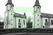
The following illustrations show a church taken from two viewpoints. The second camera position is further to the right and is a little further away from the church tower than the first. Figures 1 and 2 show prominent points and Figure 3 the result of the correspondence analysis, in which similar image sections were compared with one another - without taking into account the recording geometry. It can be clearly seen that not all correspondence was correctly identified. This is not the case especially in the area of ​​the trees, since the branches here all have a similar shape and brightness and the correspondence analysis therefore leads to incorrect results. For example, correspondences with prominent points in the tree on the right in the second image are found, although it is not visible in the other image.

• Correspondence analysis
• 

  1. Left picture with prominent points.

• 

  2. Right picture with prominent points.

• 

  3. Putative correspondence as vectors

Before the calculation, the misallocations must be excluded by means of suitable methods for separating and eliminating outliers. The so-called RANSAC algorithm is often used for this. This algorithm can detect misallocations in the pairs of points. Applied to the calculation of , it consists of the following steps: ${\displaystyle \mathbf {F} }$

1. Randomly choose 7 or 8 point correspondences from the data points. This is done in the expectation that this correspondence will be free of errors.
2. Determine from the selected correspondence using the 7 or 8 point algorithm . ${\displaystyle \mathbf {F} }$
3. Determine all corresponding points for which applies: and save them. The threshold value is necessary because, due to measurement and calculation inaccuracies, the epipolar equation is almost never exactly fulfilled. The more pairs of points satisfy the inequality, the more likely the points originally selected did not contain any misallocations. ${\displaystyle \mathbf {x} _{2}^{\text{T}}\mathbf {Fx} _{1}\leq \epsilon }$ ${\displaystyle \epsilon }$ ${\displaystyle \mathbf {x} _{2}^{\text{T}}\mathbf {Fx} _{1}=0}$
4. Repeat steps 1-3 so often that there is a sufficiently high probability that the randomly selected point correspondences will not contain any errors.

The fundamental matrix is then determined using the largest number of pairs of points from step 3 and the 8-point algorithm. A correspondence analysis can then be carried out again in which the calculated fundamental matrix is ​​used (as described, the search area for corresponding points is reduced to the epipolar line) and a lower value is accepted for the similarity measure. These last two steps can be repeated iteratively until the number of correspondences is stable. ${\displaystyle \mathbf {F} }$

The following two figures illustrate the result. The accepted correspondences are shown in Figure 1 as red vectors. In Figure 2, selected points and their epipolar lines are drawn in the right image. Correctly assigned prominent points and their epipolar lines are shown in red. Points of the correspondence analysis that do not satisfy the epipolar equation, for which the point in the right picture does not lie on the corresponding epipolar line, are shown in green. Incorrect correspondence is shown in blue. Although these points satisfy the epipolar equation and show similar image details, they are not, however, image points of the same object point. The epipole in the right picture is the intersection of the epipolar lines and is on the left outside the picture.

• Result of the calculation
• 

  1. Correspondence (red) according to RANSAC that is used for calculation. ${\displaystyle \mathbf {F} }$

• 

  2. Some epipolar lines, calculated with . ${\displaystyle \mathbf {F} }$

special cases

Special cases of epipolar geometry
On the left the camera-object configuration, on the right the two superimposed camera images a and b with the epipolar lines (red).

Special cases can arise with certain positions of the cameras in relation to one another. Two arrangements are relevant in practice, especially for machine vision:

1. If the two image planes of cameras A and B (with the same chamber constant ) are in one plane, i.e. if the recording directions are exactly parallel to each other, the epipoles shift to infinity and the epipolar lines become families of straight lines. Using homogeneous coordinates makes it particularly easy to treat these points at infinity. In the figure, the epipolar lines of the ball centers and tangents are exactly horizontal. This configuration - known as the  stereo normal case - can often be found approximately in aerial photogrammetry and stereo vision and offers the advantage in the search for correspondence that the epipolar geometry is known due to the horizontal epipolar lines and an image correspondence is only searched for in the horizontal plane, i.e. along a line of pixels in the case of digital cameras got to. The closer the objects are to the cameras, the further away the pixels are from the position in the other image: This parallax effect indicates the distance between the objects, in short: the third dimension.
   This special case also applies to human vision: Despite the mobility of the eyes, it is almost impossible to direct the eyes in directions that are not in the same plane as the line connecting the eyes. You can only look for correspondence in such directions.
2. If the two cameras are in front of each other, i.e. if they are shifted against each other in the direction of view, the epipoles shift into the center of the image; the epipolar lines therefore run outwards in a star shape, starting from the center of the image. This configuration often occurs with mobile robots when a single camera is oriented in the direction of travel and takes pictures at different times. The image correspondences are then searched for in the successive images of the camera. In this case too, the distance from the camera position can be determined from the parallax effect. When the robot pans the camera in a curve, the epipoles shift horizontally, the front to the outside of the curve and the rear to the inside, so that the special case no longer exists.

In these special cases, the correspondence search is simplified because the epipolar geometry is known. In configurations in which camera views are only approximately parallel, this state can be created by subsequently calculating normal images.

Expansion to more than two images

Trifocal geometry

The trifocal geometry is the extension of the epipolar geometry to three images. If the position of an object point is given in two images, its position in the third image is the intersection of the two epipolar lines in this image. In contrast to the image pair, there is therefore a clear result, provided the point is not in the trifocal plane (the plane formed from the three projection centers) or the three projection centers are on a line. The arrangement in which a 3D point lies on the trifocal plane is called a singular case .

It is possible to expand the epipolar geometry to more than three images. In practice, this is only common for four views. The so-called quadrifocal tensor exists here, which describes the relationship between pixels and lines between these images. For more than four views, however, no mathematical relationships were investigated, since the complexity of the modeling and calculation is significantly higher and in most applications, starting with the fifth camera, the additional information gain is only small.

Deviations from the model of the pinhole camera

The described relationship between corresponding pixels, which can be completely described by the fundamental matrix, only applies to photographs that can be modeled by a pinhole camera. If, for example, distortions occur in the imaging on the image plane or if the image surface is not a plane, these deviations must be taken into account in the epipolar geometry. In particular, the epipolar lines on which the image point corresponding to an image point in the first image is to be sought in the second image are not straight lines.

Distortion

When distortion is any deviation from the ideal imaging model of the pinhole camera. It arises from the asymmetrical position of the aperture in a lens and leads to the fact that the reproduction scale in the image changes systematically. Lenses with a symmetrical structure usually have no (radially symmetrical) distortion. The distortion must be taken into account with other lenses and corresponding accuracy requirements. The distortion can often be modeled as radial distortion ; H. it increases with the distance from the center of the distortion (usually near the center of the image).

If a camera has been calibrated accordingly and the distortion is known, the images can be corrected. These corrected images can then be used as with distortion-free images.

Under certain conditions, the distortion can be taken into account in an extended fundamental matrix. A distortion is assumed for each image, which can be described by an (unknown) parameter and which corresponds to the replacement of the flat image surface by a square surface in three-dimensional projective space. The relationship between two corresponding points is then described by a fundamental matrix with 9 degrees of freedom. ${\displaystyle 4\times 4}$

Panoramic cameras

In the case of panorama cameras that allow recordings with a large angle of view , the recording geometry cannot be modeled by a pinhole camera with a flat image surface. The description of the epipolar geometry depends on the type of panoramic camera. If the camera consists, for example, of a pinhole camera and a hyperbolic mirror, the epipolar lines form conic sections.

footnote

1. ↑ ^{a b} A straight line is defined in homogeneous coordinates by a homogeneous linear equation between the homogeneous coordinates, that is, all points that satisfy the straight line equation lie on the straight line determined by . The points of the straight line that contains two different points and are defined by the spatial product . ${\displaystyle \mathbf {x} }$ ${\displaystyle \mathbf {l} ^{\text{T}}\mathbf {x} =0}$ ${\displaystyle \mathbf {l} }$ ${\displaystyle \mathbf {x} }$ ${\displaystyle \mathbf {x} _{1}}$ ${\displaystyle \mathbf {x} _{2}}$ ${\displaystyle \det(\mathbf {x} ,\,\mathbf {x} _{1},\,\mathbf {x} _{2})\,=\,(\mathbf {x} _{1}\times \mathbf {x} _{2})^{\text{T}}\mathbf {x} \,=\,0}$

literature

• Richard Hartley, Andrew Zisserman: Multiple View Geometry in Computer Vision . 2nd Edition. Cambridge University Press, 2004, ISBN 0-521-54051-8 .
• Olivier Faugeras: Three-Dimensional Computer Vision - A Geometric Viewpoint . MIT Press, Cambridge (Massachusetts) 1993, ISBN 0-262-06158-9 .
• Volker Rodehorst: Photogrammetric 3D reconstruction at close range through auto-calibration with projective geometry . wvb Wissenschaftlicher Verlag Berlin, 2004, ISBN 3-936846-83-9 .
• Oliver Schreer: Stereo analysis and image synthesis . Springer, Berlin, 2008, ISBN 978-3-540-23439-5 .
• Richard Hartley, Andrew Zisserman: Chapter 9 from Multiple View Geometry in computer vision. (PDF; 265 kB) 2007, accessed on August 18, 2007 . 
• Zhengyou Zhang: Determining the Epipolar Geometry and its Uncertainty: A Review. (PDF; 1.6 MB) 1996, accessed on August 8, 2007 . 
• Andrew Zisserman: MATLAB Functions for Multiple View Geometry. 2007, accessed August 14, 2007 . 

Web links

• SRI International - Java applets to illustrate the imaging laws for one, two or three cameras
• University of Siena - Epipolar Geometry Toolbox ( Matlab routines)
• The Fundamental Matrix Song - A song that explains the fundamental matrix and epipolar geometry in a nutshell (by Daniel Wedge)

Individual evidence

1. ^ Karl Kraus, Peter Waldhäusl: Photogrammetrie, Volume 1 . Ferd. Dümmler, Bonn 1997, ISBN 3-427-78646-3 .
2. ↑ Ephrahim Garcia: Technical Review of Team Cornell's Spider DARPA Grand Challenge 2005 . August 28, 2005 ( darpa.mil [PDF; 1.3 MB ; accessed on July 23, 2012]).
3. ↑ Sebastian Finsterwalder: The geometric basics of photogrammetry . In: Annual report of the German Mathematicians Association . tape 6 , no. 2 . Leipzig 1899, p. 1-41 . ( Full text )
4. ↑ Horst von Sanden: The determination of the key points in photogrammetry (dissertation at the University of Göttingen) . Goettingen 1908.
5. ↑ ^{a b} H. C. Longuet-Higgins: A computer algorithm for reconstructing a scene from two projections . In: Nature . tape 293 , 1981, pp. 133-135 .
6. ↑ TS Huang, OD Faugeras: Some Properties of the E-matrix in two-view motion estimation . In: IEEE Transactions on Pattern Analysis and Machine Intelligence . tape 11 , 1989, pp. 1310-1312 .
7. ↑ BKP Horn: Relative Orientation . In: International Journal of Computer Vision . tape 4 , 1990, pp. 59-78 .
8. ↑ T. Vieville, D. Lingrand: Using singular displacements for uncalibrated monocular vision systems . In: Technical Report 2678 INRIA . 1995.
9. ↑ Zhengyou Zhang: Determining the epipolar Geometry and its Uncertainty: A Review. (PDF; 1.6 MB) 1996, accessed on August 8, 2007 . 
10. ↑ Joao P. Barreto and Kostas Daniilidis: Fundamental Matrix for Cameras with Radial Distortion . In: Proceedings of the Tenth IEEE International Conference on Computer Vision (ICCV'05) , 2005, pp. 625–632 ( PDF ( Memento of the original from June 29, 2010 in the Internet Archive ) Info: The archive link was automatically inserted and not yet checked. Please check the original and archive link according to the instructions and then remove this note. ) 

This article was added to the list of excellent articles on March 8, 2008 in this version .