Spectral clustering

Graph with two connected components

The spectral clustering is a method of cluster analysis . The objects to be clustered are viewed as nodes of a graph . The distances or dissimilarities between the objects are represented by the weighted edges between the nodes of the graph. Graph-theoretical results using Laplace matrices of graphs with connected components are the basis of spectral clustering. The eigenvalues ​​of a matrix are also called spectrum , hence the name of the method. The graph theoretical foundations were laid by Donath & Hoffman (1973) and Fiedler (1973). ${\displaystyle k}$

Mathematical basics

Graph reduction

In a first step the graph is reduced. The aim is to remove all edges with excessive weights from the graph. There are the following approaches:

${\displaystyle \epsilon }$ Neighborhood graph

If the edge weight is greater than , then this edge is removed from the graph. ${\displaystyle \epsilon }$

k-nn graphs ( nearest neighbor graphs ) ${\displaystyle k}$

All edges to a node are sorted according to the edge weight. If an edge has an edge weight that is greater than the smallest edge weight, this edge is removed from the graph. The -nn relation, however, is not symmetric; H. it can happen that the edge weight is less than the smallest edge weight to the object , but not less than the smallest edge weight to the object . One speaks of a k-nn graph if the edge remains in the graph, if for at least one of the objects or it applies that is less than the smallest edge weight for the object, i.e. H. every object has at least edges. In contrast to this, a common k-nn graph contains only the edge if it holds for both objects that it is smaller than the smallest edge weight of the objects, i.e. H. every object has at most edges. ${\displaystyle k}$ ${\displaystyle k}$ ${\displaystyle w_{ij}}$ ${\displaystyle k}$ ${\displaystyle o_{i}}$ ${\displaystyle k}$ ${\displaystyle o_{j}}$ ${\displaystyle o_{i}}$ ${\displaystyle o_{j}}$ ${\displaystyle w_{ij}}$ ${\displaystyle k}$ ${\displaystyle k}$ ${\displaystyle w_{ij}}$ ${\displaystyle k}$ ${\displaystyle k}$

Fully connected graph

With the help of a similarity function, the edge weights are calculated from the distances between the objects. An example of a similarity function is the Gaussian similarity function . The parameter controls the size of the neighborhood as well as the parameters or . ${\displaystyle s(o_{i},o_{j})=\exp(-{\tfrac {1}{2}}d^{2}(o_{i},o_{j})/\sigma ^{2})}$ ${\displaystyle \sigma }$ ${\displaystyle \epsilon }$ ${\displaystyle k}$

• 

  Position of 8 objects in a two-dimensional space.

• 

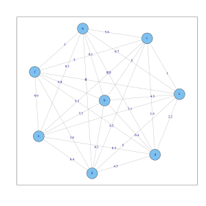
  Fully connected graph with the Euclidean distances at the edges for the 8 objects.

• 

  Distance matrix of the Euclidean distances for the 8 objects.

• 

  ${\displaystyle \epsilon }$Neighborhood graph ( ) for the 8 objects. ${\displaystyle \epsilon =5}$

• 

  k-nn Graph ( ) for the 8 objects. Every node has at least two edges. ${\displaystyle k=2}$

• 

  Common k-nn graph ( ) for the 8 objects. Each node has a maximum of two edges. The data set is broken down into 3 related components. ${\displaystyle k=2}$

• 

  Laplace matrix of the common k-nn graph ( ) for the 8 objects. ${\displaystyle L_{rw}}$ ${\displaystyle k=2}$

• 

  Fully connected graph with the values ​​of the Gaussian similarity function ( ) at the edges for the 8 objects. ${\displaystyle \sigma =3}$

Laplace matrices

The (weighted) adjacency matrix is formed for the objects from the edge weights . The diagonal matrix contains the sum of the edge weights on the diagonal, which lead to a node (after the graph reduction). Then three Laplace matrices can be calculated: ${\displaystyle n}$ ${\displaystyle W}$ ${\displaystyle D}$

• non-normalized matrix , ${\displaystyle L=D-W}$
• the normalized matrix and ${\displaystyle L_{sym}=D^{-1/2}LD^{-1/2}}$
• the normalized matrix . ${\displaystyle L_{rw}=D^{-1}L}$

The following applies to all vectors ${\displaystyle f\in R^{n}}$

${\displaystyle {\begin{array}{rcll}f^{T}Lf&=&\displaystyle {\tfrac {1}{2}}\sum _{i,j=1}^{n}w_{ij}\left(f_{i}-f_{j}\right)^{2}&\geq 0,\\f^{T}L_{sym}f&=&\displaystyle {\tfrac {1}{2}}\sum _{i,j=1}^{n}w_{ij}\left({\tfrac {f_{i}}{\sqrt {d_{i}}}}-{\tfrac {f_{j}}{\sqrt {d_{j}}}}\right)^{2}&\geq 0.\\f^{T}L_{rw}f&=&\displaystyle {\tfrac {1}{2}}\sum _{i,j=1}^{n}w_{ij}\left(f_{i}-f_{j}\right)^{2}&\geq 0\\\end{array}}}$

Since the Laplace matrices are symmetric and positive-semidefinite , all eigenvalues ​​are real-valued and greater than or equal to zero. For the Laplace matrix it can be shown that at least one eigenvalue is zero. If the graph consists of connected components, then the Laplace matrices are block matrices (see graphic and matrix above). Each block has an eigenvalue equal to zero. For the eigenvectors to the eigenvalue zero must be. Since all edge weights are positive, all entries of the nodes of a connected component must be the same (so that applies). This applies analogously to , except that the entries in the eigenvector are also weighted, while the entries in the eigenvector are equal to one. ${\displaystyle k}$ ${\displaystyle f^{T}Lf=0}$ ${\displaystyle w_{ij}}$ ${\displaystyle f_{i}}$ ${\displaystyle f_{i}-f_{j}=0}$ ${\displaystyle L_{sym}}$ ${\displaystyle d_{i}}$ ${\displaystyle L_{rw}}$ ${\displaystyle f_{i}}$

For clustering, the smallest eigenvalues ​​and vectors of the Laplace matrices are analyzed.

• 

  Eigenvalues ​​of the Laplace matrix of the common k-nn graph ( ) for the 8 objects data. Since the graph consists of three connected components, there are three eigenvalues ​​with the value zero. ${\displaystyle k=3}$

• 

  Values ​​of the three eigenvectors for the eigenvalue zero of the Laplace matrix . The entries should be equal to one, but the software rescales the eigenvectors so that they are of length one. ${\displaystyle L_{rw}}$

• 

  3D scatter plot of the three eigenvectors for the zero eigenvalues. The eight objects are plotted at three positions (overplotting), so that a k-means clustering can find the three connected components perfectly.

Algorithms

Different spectral clustering algorithms have been developed:

Non-normalized spectral clustering

1. Calculate the non-normalized Laplace matrix ${\displaystyle L}$
2. Calculate the eigenvectors for the greatest eigenvalues ${\displaystyle k}$
3. Take the rows of the eigenvectors and cluster them using a partitioning method, e.g. B. the k-means algorithm ${\displaystyle k}$

Normalized spectral clustering according to Shi and Malik

1. Calculate the normalized Laplace matrix ${\displaystyle L_{rw}}$
2. Calculate the eigenvectors for the greatest eigenvalues ${\displaystyle k}$
3. Take the rows of the eigenvectors and cluster them using a partitioning method ${\displaystyle k}$

Normalized spectral clustering according to Ng, Jordan and Weiss

1. Calculate the normalized Laplace matrix ${\displaystyle L_{sym}}$
2. Calculate the eigenvectors for the greatest eigenvalues ${\displaystyle k}$
3. Take the rows of the eigenvectors and cluster them using a partitioning method ${\displaystyle k}$

Regarding the choice of the process parameters and algorithms, the tutorial by Ulrike von Luxburg recommends :

• Choice of the neighborhood graph : the k-nn graph , as it can better recognize clusters of different densities and generates a sparse Laplace matrix . In addition, it can vary over a larger area without the cluster analysis changing significantly. ${\displaystyle k}$
• Choice of parameters of the neighborhood graph:
  • For the k-nn graph it should be chosen that the graph has no fewer connected components than one would expect clusters. ${\displaystyle k}$
  • For the common k-nn graph should be larger than for the k-nn graph , since the common k-nn graph contains fewer edges than the k-nn graph . There is no known heuristic for the choice of . ${\displaystyle k}$ ${\displaystyle k}$
  • For the neighborhood graph should be equal to the longest edge in the minimum spanning tree choose (minimal spanning tree Engl.). ${\displaystyle \epsilon }$ ${\displaystyle \epsilon }$
  • For the fully connected graph with the Gaussian similarity function, it should be chosen so that the resulting graph corresponds to the k-nn graph or the neighborhood graph . The rule of thumb is also: equal to the longest edge in the minimum spanning tree or as the mean distance to the nearest neighbor . ${\displaystyle \sigma }$ ${\displaystyle \epsilon }$ ${\displaystyle \sigma }$ ${\displaystyle \sigma }$ ${\displaystyle k}$ ${\displaystyle k=1+\log(n)}$
• Choice of number of clusters: Plot the eigenvalues ​​of the Laplace matrix, sort according to size and look for jumps, e.g. B. in the graphic above between the 3rd and 4th eigenvalue for the 8-object data set.
• Choice of the Laplace matrix: Since the entries in the eigenvector are equal to one at , z. B. the k-means algorithm cluster well. ${\displaystyle L_{rw}}$

example

The Iris data set was used by Sir Ronald Fisher (1936) as an example of a discriminant analysis . It is sometimes called 'Anderson's Iris Dataset' because Edgar Anderson collected the data to quantify the morphological variation in irises . The data set consists of 50 specimens of three species each: the bristle iris (Iris setosa), the iridescent iris (Iris versicolor) and the Virginian iris (Iris virginica). At a sepal (engl. Sepal) and at a Kronblatt the length and width were measured (engl. Petal) respectively. The data set therefore contains 150 observations and 4 variables.

• 

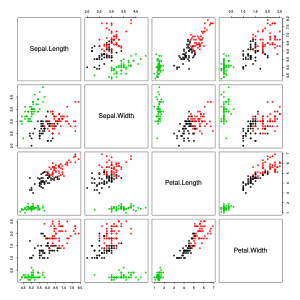
  Scatterplot matrix of the Iris dataset. The colors of the data points correspond to the three types.

• 

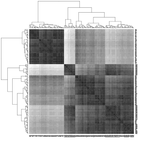
  Heat map of the Euclidean distances in the Iris dataset. The darker the color, the smaller the distance between the objects.

• 

  Result of the spectral clustering on the Iris data set.

As you can see in the left (first) graphic in the scatter diagram matrix, one of the three types (red in the graphic) differs significantly from the other types. The other two types are difficult to separate from each other. The middle (second) graphic shows the Euclidean distances between the objects in a heat map with gray levels. The darker the gray, the closer the objects are. The objects have already been rearranged in such a way that objects with similar distances to other objects are close to one another. The software used uses a hierarchical clustering method and also shows the dendrograms . The right (third) graphic shows the result of the spectral clustering. It can be seen that the clusters found agree somewhat with the three types.

• 

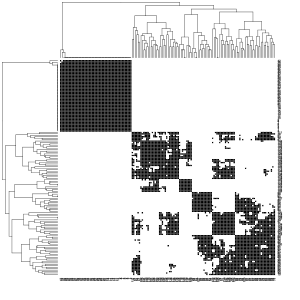
  Black: Edges between objects that are retained in a k-nn graph ( ). White: edges that have been deleted. ${\displaystyle k=50}$

• 

  Black: Edges between objects that are retained in a common k-nn graph ( ). White: edges that have been deleted. ${\displaystyle k=50}$

• 

  Scatter plot of the eigenvalues ​​of the Laplace matrix for the k-nn graph ( ). ${\displaystyle L_{rw}}$ ${\displaystyle k=50}$

The two pictures on the left show which edges in the k-nn graph or the common k-nn graph were retained (black) or not (white). For the parameter , the longest edge was first determined in a minimal spanning tree and then calculated for all observations which number of neighborhoods it corresponds to. The mean value was about 60 neighbors and it was then chosen. Then the Laplace matrix and its eigenvalues ​​were calculated. The diagram of the eigenvalues ​​shows large jumps after the second or third eigenvalue. The first three eigenvectors were then subjected to k-means clustering with 3 clusters. ${\displaystyle k}$ ${\displaystyle k=50}$ ${\displaystyle L_{rw}}$

	Cluster
Art	1	2	3
setosa	0	0	50
versicolor	43	7th	0
virginica	7th	43	0

The confusion matrix shows that spectral clustering has to some extent rediscovered the species. The Setosa cluster has been found completely correct. In the case of the Versicolor and Virginica clusters, seven observations each were classified incorrectly, which corresponds to a false classification rate of . ${\displaystyle 14/150\approx 9{,}4\,\%}$

Individual evidence

1. ^ WE Donath, AJ Hoffman: Lower bounds for the partitioning of graphs . In: IBM Journal of Research and Development. 17 (5), (1973), pp. 420-425.
2. ^ M. Fiedler: Algebraic connectivity of graphs . In: Czechoslovak Mathematical Journal. 23 (2), (1973), pp. 298-305.
3. ↑ Ulrike von Luxburg: A Tutorial on Spectral Clustering. 2007, accessed January 6, 2018 . 
4. ↑ J. Shi, J. Malik: Normalized cuts and image segmentation . In: IEEE Transactions on Pattern Analysis and Machine Intelligence. 22 (8), (2000), pp. 888-905. doi: 10.1109 / 34.868688
5. ^ AY Ng, MI Jordan, Y. Weiss: On spectral clustering: Analysis and an algorithm . In: Advances in Neural Information Processing Systems. 2, 2002, pp. 849-856.
6. ↑ Ulrike von Luxburg : A tutorial on spectral clustering. (PDF). In: Statistics and Computing. 17 (4), (2007), pp. 395-416. doi: 10.1007 / s11222-007-9033-z
7. ^ RA Fisher: The use of multiple measurements in taxonomic problems . In: Annals of Eugenics. 7 (2), (1936), pp. 179-188. doi: 10.1111 / j.1469-1809.1936.tb02137.x
8. ↑ E. Anderson: The species problem in Iris . In: Annals of the Missouri Botanical Garden. 1936, pp. 457-509.