Stability function

The stability function is an aid in numerics to analyze solution methods for ordinary differential equations . The simple test equation by Germund Dahlquist with has the exponential function as a solution . With most of the methods for ordinary differential equations, the calculated approximate solution after a time step with a step size can also be written as a function that only depends on the product . This function is the stability function and is often referred to as. A comparison with the exponential function provides basic information about the numerical method. Some stability terms refer to the properties of . ${\displaystyle y'(t)=\lambda y(t),\ y(0)=1}$ ${\displaystyle \lambda \in \mathbb {C} }$ ${\displaystyle y(t)=e^{\lambda t}}$ ${\displaystyle h}$ ${\displaystyle z=h\lambda \in \mathbb {C} }$ ${\displaystyle R(z)}$ ${\displaystyle e^{z}=e^{h\lambda }}$ ${\displaystyle R(z)}$

Stability area and terms of stability

With the aid of the stability function , the leaves stability area describe and calculate, in the form ${\displaystyle R(z)}$ ${\displaystyle S}$

${\displaystyle S=\{z\in \mathbb {C} :|R(z)|<1\}.}$

This is because in the case of one-step methods , the relationship and therefore applies to the approximations at the time ${\displaystyle y_{n}}$ ${\displaystyle t_{n}=nh}$ ${\displaystyle y_{n}=R(z)y_{n-1}=\ldots =\left(R(z)\right)^{j}y_{n-j}=\ldots =\left(R(z)\right)^{n}y_{0}}$

${\displaystyle y_{n}{\xrightarrow {n\to \infty }}0\iff z\in S.}$

If the entire left complex half-plane includes, the method is called A-stable . Then the amount of in the entire open left half-plane is less than 1. It is particularly favorable for a method if it also has the limit value 0 when it tends towards the real axis , so that the amount from there is asymptotical as the exponential function behaves. Then the procedure is called L-stable . ${\displaystyle S}$ ${\displaystyle R}$ ${\displaystyle R(z)}$ ${\displaystyle z}$ ${\displaystyle -\infty }$ ${\displaystyle R(z)}$

example

The explicit Euler method gives the test equation with after one step ${\displaystyle y_{n+1}=y_{n}+hf(t_{n},y_{n})}$ ${\displaystyle f(t,y)=\lambda y}$

${\displaystyle y_{1}=y_{0}+h\lambda y_{0}=(1+h\lambda )y_{0}}$,

thus applies to its stability function . Its area of ​​stability therefore consists of all complex numbers with , which corresponds to the interior of the circle with center and radius in the complex number plane. ${\displaystyle R(z)=1+z}$ ${\displaystyle z}$ ${\displaystyle |1+z|<1}$ ${\displaystyle -1}$ ${\displaystyle 1}$

For the implicit Euler method , however, follows with ${\displaystyle y_{n+1}=y_{n}+hf(t_{n+1},y_{n+1})}$ ${\displaystyle f(t,y)=\lambda y}$

${\displaystyle y_{1}=y_{0}+h\lambda y_{1}\iff y_{1}={\frac {1}{1-h\lambda }}y_{0}}$,

so . The stability area is now given by the condition with ${\displaystyle R(z)={\frac {1}{1-z}}}$ ${\displaystyle |{\tfrac {1}{1-z}}|<1}$

${\displaystyle |1-z|>1}$

is equivalent to what corresponds to the outside of the circle with center and radius . It therefore contains the entire open left half-plane and thus the implicit Euler method is A-stable. Because of that it is even L-stable. ${\displaystyle 1}$ ${\displaystyle 1}$ ${\displaystyle \lim _{z\to -\infty }{\frac {1}{1-z}}=0}$

The stability function of the Runge-Kutta method

Runge-Kutta methods are completely determined by the coefficients from their Butcher tableau. In the test equation is the initial value and for the levels it results in the first time step ${\displaystyle A,b,c}$ ${\displaystyle y_{0}=1}$

${\displaystyle k_{i}=\lambda \left(1+h\sum _{j=1}^{s}a_{ij}k_{j}\right),\quad i=1,\dotsc ,s.}$

This is a quadratic linear system of equations for the vector in the form with the vector. With its solution one then gets the Runge-Kutta approximation in the form ${\displaystyle k=(k_{1},\dotsc ,k_{s})^{T}}$ ${\displaystyle (I-zA)k=\lambda e}$ ${\displaystyle e=(1,\dotsc ,1)^{T}.}$ ${\displaystyle y_{1}\approx y(h)}$

${\displaystyle y_{1}=y_{0}+h\sum _{j=1}^{s}b_{j}k_{j}=1+hb^{T}k=1+zb^{T}(I-zA)^{-1}e=:R(z).}$

This is a rational function in the Runge-Kutta method, which is why it is often referred to as. ${\displaystyle R(z)}$

In the case of explicit Runge-Kutta methods, the coefficient matrix is a strictly lower triangular matrix , so the Neumann series breaks off from to s summands and you get ${\displaystyle A}$ ${\displaystyle (I-zA)^{-1}}$

${\displaystyle R(z)=1+zb^{T}(I-zA)^{-1}e=1+zb^{T}e+z^{2}b^{T}Ae+\dotsb +z^{s}b^{T}A^{s-1}e.}$

Therefore the stability function of an explicit Runge-Kutta method is a polynomial, such methods cannot be A-stable .

In the case of implicit Runge-Kutta methods , however, B. the Gauss-Legendre method A-stable . The stability functions of these special methods are even very good approximations to the exponential function , namely the so-called Padé approximations .

The stability function of multistep methods

Applying a linear multi-step procedure to the test equation results in the equation again ${\displaystyle \sum _{j=0}^{m}\alpha _{j}y_{n-j}=h\sum _{j=0}^{m}\beta _{j}f(y_{n-j})}$ ${\displaystyle z=h\lambda }$

${\displaystyle \sum _{j=0}^{m}\alpha _{j}y_{n-j}-z\sum _{j=0}^{m}\beta _{j}y_{n-j}=\sum _{j=0}^{m}(\alpha _{j}-z\beta _{j})y_{n-j}=0.}$

This is a linear difference equation that is easy to solve. Because the consequence is a nontrivial solution of this difference equation if u is a zero of the characteristic polynomial ${\displaystyle y_{n}=u^{n}}$

${\displaystyle 0{\stackrel {!}{=}}\sum _{j=0}^{m}\alpha _{j}u^{m-j}-z\sum _{j=0}^{m}\beta _{j}u^{m-j}=\varrho (u)-z\sigma (u)}$

is, where the polynomials

${\displaystyle \varrho (u)=\sum _{j=0}^{m}\alpha _{j}u^{m-j}}$

${\displaystyle \sigma (u)=\sum _{j=0}^{m}\beta _{j}u^{m-j}}$

introduced. So one gets the solutions to the test equation with the zeros of the polynomial that depend on and therefore the stability region of the method is when all these solutions approach 0 for . Therefore one can view the zero point with the maximum amount as a stability function of the method. ${\displaystyle z}$ ${\displaystyle u}$ ${\displaystyle \varrho (u)-z\sigma (u)}$ ${\displaystyle u^{n}}$ ${\displaystyle z}$ ${\displaystyle n\to \infty }$ ${\displaystyle |u(z)|}$

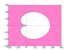
Stability area for the 6-stage BDF process

This interpretation seems very unwieldy. However, one is often less interested in the stability function than in the stability region . The edge of this area consists of the one for which the zeros apply where the zeros lie on the complex unit circle. Since it is true that the determination of the stability area is even particularly easy with multi-step methods, because its edge is obtained i. W. explicitly through ${\displaystyle S}$ ${\displaystyle z\in \mathbb {C} }$ ${\displaystyle |u|=1}$ ${\displaystyle \varrho (u)-z\sigma (u)=0\Leftarrow z=\varrho (u)/\sigma (u)}$

${\displaystyle \partial S={\Big \{}{\frac {\varrho (u)}{\sigma (u)}}:\,|u|=1{\Big \}}={\Big \{}{\frac {\varrho (e^{i\varphi })}{\sigma (e^{i\varphi })}}:\,\varphi \in [0,2\pi ){\Big \}}.}$

The stability area for the 6-step BDF process is shown as an example .

The stability function of general linear methods

Although multi-step process in the form of general linear process can be written, the structure is similar to that of the Runge-Kutta method further above . Hence, you get a similar result. The following applies to the vector of the step solutions ${\displaystyle Y}$

${\displaystyle Y=zAY+Uy^{[n-1]}\quad \Rightarrow Y=(I-zA)^{-1}Uy^{[n-1]}}$

and the time step therefore becomes

${\displaystyle y^{[n]}=zBY+Vy^{[n-1]}=(V+zB(I-zA)^{-1}U{\big )}y^{[n-1]}.}$

In each time step, the multiplication takes place with the same matrix

${\displaystyle M(z)=V+zB(I-zA)^{-1}U.}$

It therefore applies when the powers approach 0, i.e. all eigenvalues of lie within the complex unit circle. Therefore the spectral radius of can be seen here as a stability function in the definition of the stability region. ${\displaystyle y^{[n]}=M(z)^{n}y^{[0]}\to 0\,(n\to \infty )}$ ${\displaystyle M(z)}$ ${\displaystyle M(z)}$ ${\displaystyle M(z)}$ ${\displaystyle R(z)}$ ${\displaystyle S}$

Further meaning for linear systems

The above test equation by Dahlquist is very simple, but has a wider meaning for systems of linear, autonomous and homogeneous differential equations

${\displaystyle y'(t)=Qy(t),\quad y(0)=y_{0},\quad Q\in \mathbb {R} ^{d\times d}.}$

The exact solution is with the matrix exponential . The numerical solution can now be represented with the matrix stability function. If where is the Jordan normal form of , then applies ${\displaystyle y(t)=e^{tQ}y_{0}}$ ${\displaystyle e^{tQ}}$ ${\displaystyle y_{n}}$ ${\displaystyle R(tQ)}$ ${\displaystyle J=P^{-1}QP}$ ${\displaystyle Q\ (=PJP^{-1})}$

${\displaystyle y_{n}={\big (}R(hQ){\big )}^{n}y_{0}=P{\big (}R(hJ){\big )}^{n}P^{-1}y_{0}.}$

For a diagonalizable matrix , is a diagonal matrix with the diagonal elements . If that is true for all eigenvalues of , then also converges here . With this differential equation you can see at the same time that it makes sense to define it as an open set. Because in the diagonalizable case, solutions on the boundary with still remain restricted, but generally no longer if multiple eigenvalues ​​with Jordan blocks occur. ${\displaystyle Q}$ ${\displaystyle R(hJ)}$ ${\displaystyle R(h\lambda _{j})}$ ${\displaystyle \lambda _{j}}$ ${\displaystyle Q}$ ${\displaystyle h\lambda _{j}\in S}$ ${\displaystyle y_{n}\to 0\,(n\to \infty )}$ ${\displaystyle S}$ ${\displaystyle h\lambda _{j}\in \partial S}$

literature

• E. Hairer, G. Wanner: Solving Ordinary Differential Equations II, Stiff problems. Springer publishing house.
• K. Strehmel, R. Weiner, H. Podhaisky: Numerics of ordinary differential equations - non -rigid, rigid and differential-algebraic equations. Springer Spectrum, 2012.