Indifference curve

An indifference curve in the two-goods case. The amount of good 1 is plotted on the horizontal axis and that of good 2 is plotted on the vertical axis.

An indifference curve (Latin : indifferent : “not differing”; also iso-utility function , iso-utility curve and utility isoquant ) denotes the geometric location of all consumption plans with the same utility index in economics and there in particular in household theory. The indifference curve is thus the geometric location of all consumption plans between which the household is indifferent, i.e. which it assesses as equally good. It is based on the concept of the utility function , which assigns a number to any combination of quantities of goods in such a way that combinations of goods that are found by the household to be better than others are given a higher number. For each level of utility, an indifference curve can then be found on which all the bundles of goods that generate precisely this utility lie.

The term goes back to Francis Ysidro Edgeworth and was introduced into economic theory by Vilfredo Pareto to get around the problem of measuring utility . The so-called Edgeworth diagram is also based on it .

Definition and classification

Indifference curves in the three-goods case

Formal definition

If one takes a utility function as a basis, whereby the variable is referred to as utility index or simply as utility, then the indifference set (indifference curve) to the utility level is defined as the set of all tuples with which we shall say: is defined as the set of all tuples , for which the utility assumes a constant value, or to put it more banally: is defined as the set of all tuples on which the utility function assumes a certain fixed utility level. So it's short , so you can immediately see that . The indifference curve is thus a space curve in the , along which one and the same level of utility prevails. This set definition of the indifference curve also explains why the following is often referred to as equivalent to the indifference set (to a utility level), which denotes the (infinite) set of points on an indifference curve. ${\ displaystyle u (\ mathbf {x}) = u (x_ {1}, \ ldots, x_ {n})}$ ${\ displaystyle u}$ ${\ displaystyle I_ {a}}$ ${\ displaystyle {\ overline {u}} = a}$ ${\ displaystyle \ mathbf {x}}$ ${\ displaystyle u (\ mathbf {x}) = a}$ ${\ displaystyle \ mathbf {x}}$ ${\ displaystyle \ mathbf {x}}$ ${\ displaystyle I_ {a} \ equiv \ {\ mathbf {x} | u (\ mathbf {x}) = a \}}$ ${\ displaystyle I_ {a} \ subset \ mathbb {R} ^ {n}}$ ${\ displaystyle \ mathbb {R} ^ {n}}$

In the following, however, the size of the bundle of goods is often limited to two goods for reasons of simpler handling and graphical representation.

Construction in the two-goods case

Three indifference curves in the two-goods case.

To construct the indifference curves, in the two-goods case, for example, the amount of consumption of good 1 is shown on the horizontal axis of a coordinate system and the amount of consumption of good 2 is shown on the vertical axis. Assuming that both goods are infinitely divisible, one can draw an infinite number of points in the coordinate system between which the individual is indifferent. The resulting curve is the indifference curve sought.

In the example opposite, three indifference curves are drawn. Given that the corresponding utility function can be constructed indifference curves for any utility level , there are also an infinite number of conceivable indifference curves. If one assumes that a household strictly prefers bundles of goods that contain more of both goods to those with smaller quantities of goods (this is the monotonicity property, which will be more formally defined later), then the further the indifference curve from the origin, the greater the utility level away. Correspondingly, points (bundles of goods) on the indifference curve are strictly better than on and points (bundles of goods) on are strictly better than those on . Goods bundle A is valued the least, D the most. B and C are on the same indifference curve, which means that the household does not care whether it consumes bundle B or C. ${\ displaystyle u (\ mathbf {x})}$ ${\ displaystyle {\ overline {u}}}$ ${\ displaystyle I_ {3}}$ ${\ displaystyle I_ {2}}$ ${\ displaystyle I_ {2}}$ ${\ displaystyle I_ {1}}$

Assumptions and properties

Since, by definition, indifference curves reflect the subjective preferences of a household, the properties of the indifference curves are determined by this household. If one makes certain (basic) assumptions about the behavior of households, one can draw conclusions about the general properties of indifference curves. The following assumptions are usually made:

Monotony (unsaturation)

For each bundle of goods, it is assumed that the household has not reached the saturation limit for any good (this assumption makes particular sense if the household income is assumed to be so low that the unsaturation assumption is fulfilled for all consumer goods). It is always assumed that a household would rather consume more goods than less. The assumption of monotony is often interpreted as the unsaturation of the consumer: a bundle of goods like D in the figure above, which contains more of both goods than bundle A, is always preferred by the household to bundle A, both cannot lie on the same indifference curve. From this it follows immediately that if this assumption of monotonicity is valid, indifference curves (as in the figure above) must have a negative slope ( including 0). ${\ displaystyle - \ infty}$

The assumption of unsaturation is often criticized as being unrealistic. However, one can address the concerns by making the weaker assumption that no saturation can occur in all goods . In the case of this weaker assumption, the results do not change significantly.

completeness

It is assumed that the order of preference is complete; H. the household can state for any pair of goods bundles whether the alternative is better ( ), worse ( ) or equally good ( ) as the initial situation. ${\ displaystyle \ succ}$ ${\ displaystyle \ prec}$ ${\ displaystyle \ sim}$

Transitivity (or consistency)

Two intersecting “indifference curves” - transitivity assumption violated

An important property of the indifference curves can already be seen from the graphic above: indifference curves cannot intersect one another (just as contour lines on a “real” mountain cannot intersect one another). This corresponds to the principle that the hierarchy of the bundles of goods must be free of contradictions (transitivity). If a complete mountain of benefits is to be represented, then this consists of an infinitely large family of indifference curves.

In the figure, point A is indifferent to point B and point B is indifferent to point C. The principle of transitivity implies that point A must therefore also be indifferent to point C. Since these do not lie on the same indifference curve in the present example, the assumption does not apply.

Rational choice

The household decides on an optimal consumption plan in the context of its personal benefit maximization, taking into account the secondary conditions ( budget restriction , goods prices): If any consumption plan is selected from the budget, this plan is preferred to all other consumption plans (otherwise it would not have been selected ).

continuity

This is a very formal assumption, but it is needed to ensure the existence of indifference curves. This assumption ensures that the order of preference has no jumps and that the utility index function is continuously differentiable. The assumption of continuity assumes any divisibility of the goods.

Assuming - as in the figure - three alternatives A, B and D, in which B is preferred to A and D to B, then it should be in the convex combination of A and D (i.e. the straight line between A and D) always give a point that is indifferent to B.

This assumption is not fulfilled in the lexicographical order of preference . With this order of preference there are no indifference curves.

substitution

It is assumed that the indifference curves do not touch the axes of consumption levels. With this assumption, it can be ruled out that consumer goods are completely substituted (this is only plausible, however, in the case of absolutely indispensable consumer goods, such as water and bread). This assumption facilitates the calculation of optimal consumption plans (but is not necessary for the calculation).

Convexity (or balance)

In general cases, convex indifference curves are usually assumed; these guarantee a negative substitution effect . Cobb-Douglas utility functions are particularly often assumed.

In the figure, the indifference curves are convex . The shape of the indifference curves indicates in what form the household is prepared to substitute good 1 for good 2. The amount of inclination of the curve at the individual points indicates how many units of good 1 are required in exchange for one unit of good 2 in order to remain at the same level. This is called the marginal rate of substitution . If one runs through one of the indifference curves from top to bottom, as in the example, more is consumed by good 1 and less by good 2 , without the benefit achieved changing: Good 2 is substituted by good 1 if the benefit remains constant . This is the law of the decreasing marginal rate of substitution.

If a lot has been substituted for a good, it is relatively scarce. That is why many units of the other good are required for substitution. The resulting convex curve shows that the household prefers bundles of goods with mixed contents to those that contain a lot of good 1 or good 2 on one side. This can be shown in the graphic by drawing a connecting line between points B and C. The household would prefer any point on this line to points B or C, as these are on higher indifference curves. (Rule: "Mixing things up makes the household better.")

A distinction can also be made between strong and strict convexity (as in the example above), in this case balanced consumption bundles are strictly preferred, i.e. they always achieve a higher level of utility than less balanced bundles of goods. If there is only convexity (also referred to as weak convexity), the corresponding indifference curves have a section with a constant slope. Here balanced ones are no longer necessarily preferred. In the above example this would mean that points B and C as well as the points on the line connecting them lie on the same indifference curve, the consumer is then indifferent.

proof

Proof of the convexity of indifference curves:

proof
Condition for convexity ${\ displaystyle {\ frac {d ^ {2} x_ {1}} {dx_ {2} ^ {2}}} \ geq 0}$ in which ${\ displaystyle {\ frac {dx_ {1}} {dx_ {2}}} = - {\ frac {f_ {2} (\ varphi (x_ {2}), x_ {2}))} {f_ {1 } (\ varphi (x_ {2}), x_ {2}))}}}$ and ${\ displaystyle \ varphi (x_ {2}) = x_ {1}}$ ${\ displaystyle \ Rightarrow {\ frac {d ^ {2} x_ {1}} {dx_ {2} ^ {2}}} = - {\ frac {[f_ {1} \ cdot (f_ {12} \ cdot \ varphi '(x_ {2}) + f_ {22}) - f_ {2} \ cdot (f_ {11} \ cdot \ varphi' (x_ {2}) + f_ {12})]} {f_ {1 } ^ {2}}}> 0 \ \| \ cdot f_ {1} ^ {3}}$ applies here ${\ displaystyle f_ {12} = f_ {21} \!}$ and ${\ displaystyle \ varphi '(x_ {2}) = - {\ frac {f_ {2}} {f_ {1}}}}$ ${\ displaystyle \ Rightarrow 2 \ cdot f_ {12} f_ {1} f_ {2} - (f_ {1} ^ {2} f_ {22} + f_ {2} ^ {2} f_ {11})> 0 }$ applies there ${\ displaystyle f_ {12}> 0, \ f_ {22} <0, \ f_ {11} <0}$ .

Examples

Linear indifference curves - perfect substitute

Perfect complements

Indifference curves can also be linear . This means that the household is ready to swap good 1 and good 2 along the entire curve at a fixed ratio. One speaks of “ perfect substitutes ”. These are goods that can easily be exchanged for one another - for which the household does not care whether it consumes more of good 1 or more of good 2.

Perfect complements are another special form. Here the indifference curves have a kink (L-shaped). This means that the consumer wants to consume good 1 and good 2 in a fixed ratio. If you give him only one of the two goods, this does not increase his usefulness. An example of this are left and right shoes. If you buy five left and five right shoes, buying 5 more left shoes does not bring any additional benefit.

Exceptional forms of indifference curves

The following forms do not conform to the standard assumptions:

Concave indifference curves indicate that the household prefers bundles of goods that contain a lot of one of the two goods on one side. (Rule: "Extremes are preferred.") Examples are locally bound goods: A household that owns a plot of 300 m² in Berlin and another 300 m² in Munich, on the other hand, will usually have a single 600 m² in one of the prefer both cities.

Circular or elliptical indifference curves are also conceivable. There is a central point here, which lies in the middle of the round indifference curves. At this “bliss point” the household has reached its maximum level of utility. A household with such a preference order will then not trade in scarce goods (which are not available in the “bliss point”) for other scarce goods. The budget is therefore irrelevant to a price theory.

Range of benefits

Play media file

Utility mountain range of a Cobb-Douglas utility function (animation).

Each point in the indifference curve system can be assigned a utility index that fulfills the following conditions, but is otherwise arbitrary:

Two points between which the household is indifferent, i.e. which are on the same indifference curve, receive the same utility index.
If one combination is preferred to another, it receives a higher utility index.

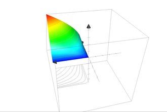
Then you can add the utility index as a third dimension to a three-dimensional coordinate system. If you determine the utility index for all possible bundles of goods from good 1 and good 2 , you get a mountain of benefits or a mountain of benefits . The indifference curve results in a utility mountain as a contour line . It comes about through a horizontal cut in the mountains. Note that, depending on the utility index selected, you get different mountains, but that they all have the same indifference curve system.

Income mountains

The yield range is the graphically displayed yield depending on two production factors and the output volume . The two production factors can be substituted and thus form an isoquant .

Household optimum

Slope of the indifference curve and marginal rate of substitution

Household optimum in the two-goods case

The marginal rate of substitution or the slope of the indifference curve denotes the exchange ratio between the goods at which the supply level does not change from the perspective of the household, i.e. subjectively. With the optimal consumption decision of a household (the household optimum), the marginal rate of substitution has the same value as the slope of the budget line (illustrated in the following example). This means that the indifference curve and the budget line touch (do not intersect) at this point. ${\ displaystyle {\ tfrac {\ mathrm {d} \, x_ {2}} {\ mathrm {d} \, x_ {1}}}}$ ${\ displaystyle {\ tfrac {-p_ {1}} {p_ {2}}}}$

Marginal rate of substitution (1st derivative of the indifference function) = price ratio (1st derivative of the budget line )

This results in the validity of Gossen's 2nd law .

Example in the two-goods case

Here the indifference curve is the highest possible indifference curve that the consumer can achieve. The consumer would prefer points on the indifference curve , but they cannot afford the combination of kebab and lemonade that is shown. In contrast, he can afford the point on the indifference curve , but he will not choose it because the curve measures a lower benefit to the consumer. ${\ displaystyle I_ {2}}$ ${\ displaystyle I_ {3}}$ ${\ displaystyle 1}$

analogy

The same point of view is also possible in production theory with different combinations of two input factors that are substituted for one another while the production level remains the same. What represents the indifference curve in household theory can be compared with the isoquant in production theory.

literature

Friedrich Breyer: Microeconomics. An introduction. 3. Edition. Springer, Heidelberg et al. 2007, ISBN 978-3-540-69230-0 , chapter 4.2.
Vilfredo Pareto: Manuale di economia politica. Milan 1906. (No German edition, the relevant remarks by Paretos from Chapter III, §§ 52-67 in German translation in W. Reiss: Mikroökonomischeorie . Oldenbourg Verlag, Munich 1992, ISBN 3-486-22277-5 , Chap. 5.).
Hal R. Varian : Fundamentals of Microeconomics . Oldenbourg Verlag, 2003, ISBN 3-486-27453-8 , chapter 3.3.
Jochen Schumann, Ulrich Meyer, Wolfgang Ströbele: Basics of the microeconomic theory. 8th edition. Springer-Verlag, Berlin et al. 2007, ISBN 978-3-540-70925-1 .

Individual evidence

^ Jörg Beutel : Microeconomics. Oldenbourg Verlag, 2006., ISBN 978-3-486-59944-2 (accessed from De Gruyter Online). P. 46
^ Jörg Beutel: Microeconomics. Oldenbourg Verlag, 2006., ISBN 978-3-486-59944-2 (accessed from De Gruyter Online). P. 42
↑ Horst Demmler: Fundamentals of microeconomics. Walter de Gruyter GmbH & Co KG, 2015. p. 12
^ Jörg Beutel: Microeconomics. Oldenbourg Verlag, 2006., ISBN 978-3-486-59944-2 (accessed from De Gruyter Online). P. 43
^ Jörg Beutel: Microeconomics. Oldenbourg Verlag, 2006., ISBN 978-3-486-59944-2 (accessed from De Gruyter Online). P. 45
^ Jörg Beutel: Microeconomics. Oldenbourg Verlag, 2006., ISBN 978-3-486-59944-2 (accessed from De Gruyter Online). P. 46
↑ Evidence from: Schumann / Meyer / Ströbele 2007, p. 55. Here presented in more detail.

Web links

Indifference curves - Article at mikrooekonomie.de
The marginal rate of substitution articles at mikrooekonomie.de (deals with special cases of indifference curves)
Indifference curve - definition in the Gabler Wirtschaftslexikon

[1] Jörg Beutel : Microeconomics. Oldenbourg Verlag, 2006., ISBN 978-3-486-59944-2 (accessed from De Gruyter Online). P. 46

[2] Jörg Beutel: Microeconomics. Oldenbourg Verlag, 2006., ISBN 978-3-486-59944-2 (accessed from De Gruyter Online). P. 42

[3] Horst Demmler: Fundamentals of microeconomics. Walter de Gruyter GmbH & Co KG, 2015. p. 12

[4] Jörg Beutel: Microeconomics. Oldenbourg Verlag, 2006., ISBN 978-3-486-59944-2 (accessed from De Gruyter Online). P. 43

[5] Jörg Beutel: Microeconomics. Oldenbourg Verlag, 2006., ISBN 978-3-486-59944-2 (accessed from De Gruyter Online). P. 45

[6] Jörg Beutel: Microeconomics. Oldenbourg Verlag, 2006., ISBN 978-3-486-59944-2 (accessed from De Gruyter Online). P. 46

[SMS-S.55-7] Evidence from: Schumann / Meyer / Ströbele 2007, p. 55. Here presented in more detail.