Airy stress function

The Airy stress function - named after George Biddell Airy - is a function from which analytical solutions for boundary value problems of linear planar elastostatics can be derived. The Airy stress function is based on the assumption of linear elasticity, small displacements and static, time-independent stresses in the plane. Finding a solution to the boundary value problem shifts to finding a stress function that satisfies the boundary conditions. Many examples and approach functions are known from the literature, with the help of which the construction of a solution is simplified.

The stresses in the plane are calculated from derivatives of the stress function, hence their name. Via the linear elasticity, the stresses are followed by the strains, from which the displacements in the plane are calculated. The success of this procedure is assured if the stress function fulfills the so-called biharmonic differential equation, disk equation or bipotential equation, which represents a partial differential equation of the 4th order. Then there is equilibrium and the calculated strains are compatible , which means that the displacements can actually be constructed from them.

To find the solution, the boundary conditions must first be formulated, which must not depend on the time due to the restriction to the statics. Both stress boundary conditions (area-distributed forces) and displacement boundary conditions can be specified. From the pool of solution functions of the disk equation known from the literature, a set is selected that fulfills these boundary conditions and the parameters of the functions are adapted to the specifications.

The Airy's stress function is of practical importance in the calculation of straight or flat construction elements (bars, beams, discs) which are widely used in mechanical engineering and structural engineering. Here the deformations are often small or have to be kept small for safety reasons. The materials used often show a linear elastic behavior up to certain application limits to a good approximation. The formulas known in technical mechanics for the elongation of the straight rod, the bending of the straight beam and the disk theory can also be represented with the Airy stress function. But it is mainly used in other problems such as B. the bending of the rod-shaped circular ring, the load on the disc with a hole or the plane with a slot (Griffith crack).

The Beltrami stress functions are the generalization of Airy's stress function to three dimensions.

requirements

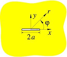
The definitions presented here are common and no special assumptions for the construction of the stress function. A plane surface carrier lying in the xy plane of a Cartesian coordinate system is considered.

kinematics

Displacements in the xy plane

The displacements of each point in the plane of the surface support is described by two functions. According to the prerequisite, the carrier lies in the xy-plane and there it is common to designate the shift in the x-direction with , that in the y-direction with and that in the z-direction with , see picture. The functions and are dependent on the location coordinates. The application here is limited to , and with a constant . Other dependencies are neglected here. In the xy-plane (small) shifts are allowed, perpendicular to them only proportionally. The pane level is included so that the pane cannot bend or move in the z-direction as a whole. These are common assumptions in disk theory. ${\displaystyle u}$ ${\displaystyle v}$ ${\displaystyle w}$ ${\displaystyle u,v}$ ${\displaystyle w}$ ${\displaystyle u=u(x,y)}$ ${\displaystyle v=v(x,y)}$ ${\displaystyle w=z\varepsilon _{zz}}$ ${\displaystyle \varepsilon _{zz}}$ ${\displaystyle \varepsilon _{zz}}$ ${\displaystyle z=0}$

The expansions describe how much the displacements change from one place to another: Places where the displacements change strongly have large expansions. Accordingly, it makes sense to calculate the strains from the derivatives according to the location. In the geometrically linear case here the only relevant expansion components are:

${\displaystyle \varepsilon _{xx}={\frac {\mathrm {d} u}{\mathrm {d} x}}\,,\varepsilon _{yy}={\frac {\mathrm {d} v}{\mathrm {d} y}}\,,\varepsilon _{zz}={\frac {\mathrm {d} w}{\mathrm {d} z}}\quad \mathrm {und} \quad \varepsilon _{xy}={\frac {1}{2}}\left({\frac {\mathrm {d} u}{\mathrm {d} y}}+{\frac {\mathrm {d} v}{\mathrm {d} x}}\right)}$.

The functions and are the normal strains in the x, y and z directions and are the shear distortion in the xy plane. Other expansion components (possible in three dimensions) disappear depending on the assumption. ${\displaystyle \varepsilon _{xx}\,,\varepsilon _{yy}}$ ${\displaystyle \varepsilon _{zz}}$ ${\displaystyle \varepsilon _{xy}}$

Flat state of stress and strain

Panes are flat surface carriers that are only loaded in their plane. Rods and beams are included in this consideration as a special case of the narrow and thin disk. If there are no loads perpendicular to the plane, there is a plane stress state (ESZ) in the pane. Surface beams that are also loaded perpendicular to their plane are called plates. If this plate is so thick that it is not noticeably compressed by the load acting on it perpendicularly, a level state of distortion prevails in its plane (EVZ). In the plane stress state, all stress components are negligibly small, and in the plane distortion state all strain components perpendicular to the plane of the surface support are negligibly small.

Linear elasticity

→ Main article : Hooke's law

With a linear elastic body, the stresses in the ESZ depend on the strains according to the following matrix equation : ${\displaystyle \sigma _{ij}}$ ${\displaystyle \varepsilon _{ij}}$

${\displaystyle {\begin{pmatrix}\sigma _{xx}\\\sigma _{yy}\\\sigma _{xy}\end{pmatrix}}={\frac {E}{1-\nu ^{2}}}{\begin{pmatrix}1&\nu &0\\\nu &1&0\\0&0&1-\nu \end{pmatrix}}{\begin{pmatrix}\varepsilon _{xx}\\\varepsilon _{yy}\\\varepsilon _{xy}\end{pmatrix}}\quad \Leftrightarrow \quad {\begin{pmatrix}\varepsilon _{xx}\\\varepsilon _{yy}\\\varepsilon _{xy}\end{pmatrix}}={\frac {1}{E}}{\begin{pmatrix}1&-\nu &0\\-\nu &1&0\\0&0&1+\nu \end{pmatrix}}{\begin{pmatrix}\sigma _{xx}\\\sigma _{yy}\\\sigma _{xy}\end{pmatrix}}}$

The parameter is the modulus of elasticity and the Poisson's ratio . The zz component of the elongation results in ${\displaystyle E}$ ${\displaystyle \nu }$

${\displaystyle \varepsilon _{zz}=-{\frac {\nu }{1-\nu }}(\varepsilon _{xx}+\varepsilon _{yy})=-{\frac {\nu }{E}}(\sigma _{xx}+\sigma _{yy})}$.

There is a constant on the left side of the equation, but mostly not on the right side. Therefore, the ESZ will generally only be met approximately. The following applies in the EVZ

${\displaystyle {\begin{pmatrix}\sigma _{xx}\\\sigma _{yy}\\\sigma _{xy}\end{pmatrix}}={\frac {2G}{1-2\nu }}{\begin{pmatrix}1-\nu &\nu &0\\\nu &1-\nu &0\\0&0&1-2\nu \end{pmatrix}}{\begin{pmatrix}\varepsilon _{xx}\\\varepsilon _{yy}\\\varepsilon _{xy}\end{pmatrix}}\quad \Leftrightarrow \quad {\begin{pmatrix}\varepsilon _{xx}\\\varepsilon _{yy}\\\varepsilon _{xy}\end{pmatrix}}={\frac {1}{2G}}{\begin{pmatrix}1-\nu &-\nu &0\\-\nu &1-\nu &0\\0&0&1\end{pmatrix}}{\begin{pmatrix}\sigma _{xx}\\\sigma _{yy}\\\sigma _{xy}\end{pmatrix}}}$

with the zz component of the voltage

${\displaystyle \sigma _{zz}=\nu (\sigma _{xx}+\sigma _{yy})=\lambda (\varepsilon _{xx}+\varepsilon _{yy})}$

where the Lame constant was used. ${\displaystyle \lambda ={\tfrac {\nu E}{(1+\nu )(1-2\nu )}}}$

The following relationships can be seen from this:

${\displaystyle {\begin{array}{l}\varepsilon _{xx}=a\sigma _{xx}-b\sigma _{yy}\\\varepsilon _{yy}=a\sigma _{yy}-b\sigma _{xx}\\\varepsilon _{xy}={\frac {\sigma _{xy}}{2G}}\end{array}}}$

With

size	Flat state of distortion (EVZ)	Plane stress state (ESZ)
${\displaystyle a}$	${\displaystyle {\frac {1-\nu }{2G}}}$	${\displaystyle {\frac {1}{E}}}$
${\displaystyle b}$	${\displaystyle {\frac {\nu }{2G}}}$	${\displaystyle {\frac {\nu }{E}}}$
${\displaystyle 2Ga,1-2Gb}$	${\displaystyle 1-\nu }$	${\displaystyle {\frac {1}{1+\nu }}}$

By replacing through , the formulas for the ETC are transferred to those for the ESZ. ${\displaystyle \nu }$ ${\displaystyle \nu ^{\ast }={\frac {\nu }{1+\nu }}}$

Compatibility condition

→ Main article : Compatibility condition

If the displacements are to be determined from the distortions, which is the case here, only two displacements and have to be calculated from the three distortions and , so the distortions cannot be independent of one another. The compatibility condition ensures that the displacements can be reconstructed from the distortions. The shear distortions are derived from x and y and the normal strains are used ${\displaystyle \varepsilon _{xx},\varepsilon _{yy}}$ ${\displaystyle \varepsilon _{xy}}$ ${\displaystyle u}$ ${\displaystyle v}$ ${\displaystyle \varepsilon _{xy}}$

${\displaystyle 2{\frac {\mathrm {d} ^{2}\varepsilon _{xy}}{\mathrm {d} x\mathrm {d} y}}={\frac {\mathrm {d} ^{3}u}{\mathrm {d} x\mathrm {d} ^{2}y}}+{\frac {\mathrm {d} ^{3}v}{\mathrm {d} {x}^{2}\mathrm {d} y}}={\frac {\mathrm {d} ^{2}\varepsilon _{xx}}{\mathrm {d} {y}^{2}}}+{\frac {\mathrm {d} ^{2}\varepsilon _{yy}}{\mathrm {d} {x}^{2}}}}$.

This is the compatibility condition for the expansion in the two-dimensional case. If the strains are replaced by the stresses and the equation multiplied by, the result is: ${\displaystyle G}$

${\displaystyle {\frac {\mathrm {d} ^{2}\sigma _{xy}}{\mathrm {d} x\mathrm {d} y}}=G{\frac {\mathrm {d} ^{2}(a\sigma _{xx}-b\sigma _{yy})}{\mathrm {d} {y}^{2}}}+G{\frac {\mathrm {d} ^{2}(a\sigma _{yy}-b\sigma _{xx})}{\mathrm {d} {x}^{2}}}=G\left(a{\frac {\mathrm {d} ^{2}}{\mathrm {d} {y}^{2}}}-b{\frac {\mathrm {d} ^{2}}{\mathrm {d} {x}^{2}}}\right)\sigma _{xx}+G\left(a{\frac {\mathrm {d} ^{2}}{\mathrm {d} {x}^{2}}}-b{\frac {\mathrm {d} ^{2}}{\mathrm {d} {y}^{2}}}\right)\sigma _{yy}}$.

balance

→ Main article : Mechanical balance

Stresses on a disc element

In equilibrium, the forces on a disk element cancel each other out in the x and y directions:

${\displaystyle {\begin{array}{l}\sigma _{xx}(x+{\text{d}}x,y){\text{d}}y+\sigma _{xy}(x,y+{\text{d}}y){\text{d}}x-\sigma _{xx}(x,y){\text{d}}y-\sigma _{xy}(x,y){\text{d}}x=0\\\sigma _{yy}(x,y+{\text{d}}y){\text{d}}x+\sigma _{xy}(x+{\text{d}}x,y){\text{d}}y-\sigma _{yy}(x,y){\text{d}}x-\sigma _{xy}(x,y){\text{d}}y=0\\\end{array}}}$

see image. Division by yields in the limit value and the equilibrium condition in the x or y direction: ${\displaystyle {\text{d}}x{\text{d}}y}$ ${\displaystyle {\text{d}}x\rightarrow 0}$ ${\displaystyle {\text{d}}y\rightarrow 0}$

${\displaystyle {\begin{array}{c}{\frac {\mathrm {d} \sigma _{xx}}{\mathrm {d} x}}+{\frac {\mathrm {d} \sigma _{xy}}{\mathrm {d} y}}=0\\{\frac {\mathrm {d} \sigma _{yy}}{\mathrm {d} y}}+{\frac {\mathrm {d} \sigma _{xy}}{\mathrm {d} x}}=0\end{array}}}$.

Differentiation of the upper equation according to x, the lower equation according to y, addition of the resulting equations and insertion of the compatibility condition expressed in stresses leads to ${\displaystyle 2Ga=1-2Gb}$

${\displaystyle {\begin{array}{rcl}{\frac {\mathrm {d} ^{2}\sigma _{xx}}{\mathrm {d} x^{2}}}+{\frac {\mathrm {d} ^{2}\sigma _{yy}}{\mathrm {d} y^{2}}}+2{\frac {\mathrm {d} \sigma _{xy}}{\mathrm {d} x\mathrm {d} y}}&=&{\frac {\mathrm {d} ^{2}\sigma _{xx}}{\mathrm {d} x^{2}}}+{\frac {\mathrm {d} ^{2}\sigma _{yy}}{\mathrm {d} y^{2}}}+2\left[G\left(a{\frac {\mathrm {d} ^{2}}{\mathrm {d} {y}^{2}}}-b{\frac {\mathrm {d} ^{2}}{\mathrm {d} {x}^{2}}}\right)\sigma _{xx}+G\left(a{\frac {\mathrm {d} ^{2}}{\mathrm {d} {x}^{2}}}-b{\frac {\mathrm {d} ^{2}}{\mathrm {d} {y}^{2}}}\right)\sigma _{yy}\right]\\&=&(1-2Gb){\frac {\mathrm {d} ^{2}\sigma _{xx}}{\mathrm {d} x^{2}}}+(1-2Gb){\frac {\mathrm {d} ^{2}\sigma _{yy}}{\mathrm {d} y^{2}}}+2Ga{\frac {\mathrm {d} ^{2}\sigma _{xx}}{\mathrm {d} {y}^{2}}}+2Ga{\frac {\mathrm {d} ^{2}\sigma _{yy}}{\mathrm {d} {x}^{2}}}=0\\\rightarrow \left({\frac {\mathrm {d} ^{2}}{\mathrm {d} {x}^{2}}}+{\frac {\mathrm {d} ^{2}}{\mathrm {d} {y}^{2}}}\right)(\sigma _{xx}+\sigma _{yy})&=&\Delta (\sigma _{xx}+\sigma _{yy})=0\end{array}}}$

with the Laplace operator

${\displaystyle \Delta ={\frac {\mathrm {d} ^{2}}{\mathrm {d} {x}^{2}}}+{\frac {\mathrm {d} ^{2}}{\mathrm {d} {y}^{2}}}}$.

Airy's stress function

Cartesian coordinates

The stress components result from the derivation of the Airy stress function : ${\displaystyle F}$

${\displaystyle \sigma _{xx}={\frac {\mathrm {d} ^{2}{F}}{\mathrm {d} {y}^{2}}},\quad \sigma _{yy}={\frac {\mathrm {d} ^{2}{F}}{\mathrm {d} {x}^{2}}},\quad \sigma _{xy}={\frac {-\mathrm {d} ^{2}{F}}{\mathrm {d} x\mathrm {d} y}}}$.

Then the equilibrium conditions are fulfilled identically and the compatibility condition yields, for homogeneous, isotropic , linearly elastic material

${\displaystyle \Delta (\sigma _{xx}+\sigma _{yy})=\Delta \left({\frac {\mathrm {d} ^{2}{F}}{\mathrm {d} {y}^{2}}}+{\frac {\mathrm {d} ^{2}{F}}{\mathrm {d} {x}^{2}}}\right)=0}$

or

${\displaystyle \Delta \Delta F=0}$

This is the disk equation or bipotential equation . Any function that satisfies this equation is called biharmonic . Polynomials, logarithmic functions as well as products of exponential and trigonometric functions are mainly used for their solution, a selection of which is given here:

${\displaystyle {\begin{array}{lllll}1,&x,&x^{2},&x^{3}&\\xy,&x^{2}y,&x^{3}y,&x^{4}y-x^{2}y^{3},&x^{4}-3x^{2}y^{2}\\x^{5}-5x^{3}y^{2},&x^{5}y-5/3x^{3}y^{3},&x^{6}-10x^{4}y^{2}+5x^{2}y^{4}&&\\e^{\pm \lambda y}\cos(\lambda x),&xe^{\pm \lambda y}\cos(\lambda x),&\cosh(\lambda x)\cos(\lambda x),&x\cosh(\lambda x)\cos(\lambda x)&\\\ln(x^{2}+y^{2}),&x\ln(x^{2}+y^{2}).&&&\\\end{array}}}$

In these terms, x and y, sin and cos and sinh and cosh can be interchanged.

Orthotropy

→ Main article : Orthotropy

For homogeneous, orthotropic , linearly elastic material, the descriptive differential equation results as:

${\displaystyle {\frac {\mathrm {d} ^{4}{F}}{\mathrm {d} {x}^{4}}}+\left({\frac {E_{y}}{G_{xy}}}-2\cdot \nu _{yx}\right)\cdot {\frac {\mathrm {d} ^{4}{F}}{\mathrm {d} {x}^{2}\cdot \mathrm {d} {y}^{2}}}+{\frac {E_{y}}{E_{x}}}\cdot {\frac {\mathrm {d} ^{4}{F}}{\mathrm {d} {y}^{4}}}}$

The disk equation remains valid when the plane is parameterized with polar coordinates or complex numbers.

Polar coordinates

The points in the xy plane can alternatively also be addressed in polar coordinates . When the above formulas are expressed in polar coordinates, the Laplace operator is:

${\displaystyle \Delta ={\frac {\mathrm {d} ^{2}}{\mathrm {d} {r}^{2}}}+{\frac {1}{{r}^{2}}}{\frac {\mathrm {d} ^{2}}{\mathrm {d} \varphi ^{2}}}+{\frac {1}{r}}{\frac {\mathrm {d} }{\mathrm {d} r}}}$.

The radius is the distance from the origin and the counterclockwise angle from the x-axis to a point in the plane. The stresses are determined in polar coordinates from the Airy stress function as follows: ${\displaystyle r}$ ${\displaystyle \varphi }$

${\displaystyle {\begin{array}{l}\sigma _{rr}={\frac {1}{{r}^{2}}}{\frac {\mathrm {d} ^{2}{F}}{\mathrm {d} \varphi ^{2}}}+{\frac {1}{r}}{\frac {\mathrm {d} {F}}{\mathrm {d} r}}\\\sigma _{\varphi \varphi }={\frac {\mathrm {d} ^{2}{F}}{\mathrm {d} {r}^{2}}}\\\sigma _{r\varphi }=-{\frac {\mathrm {d} }{\mathrm {d} r}}\left({\frac {1}{r}}{\frac {\mathrm {d} {F}}{\mathrm {d} \varphi }}\right)\end{array}}}$.

John Henry Michell found that all of the functions satisfying the disk equation have the following form:

${\displaystyle {\begin{array}{lcl}F&=&A_{0}~r^{2}+B_{0}~r^{2}~\ln(r)+C_{0}~\ln(r)+D_{0}~\varphi \\&&\displaystyle +(A_{1}~r+B_{1}~r^{-1}+B_{1}^{'}~r~\varphi +C_{1}~r^{3}+D_{1}~r~\ln(r))\cos \varphi \\&&\displaystyle +(E_{1}~r+F_{1}~r^{-1}+F_{1}^{'}~r~\varphi +G_{1}~r^{3}+H_{1}~r~\ln(r))\sin \varphi \\&&\displaystyle +\sum _{n=2}^{\infty }(A_{n}~r^{n}+B_{n}~r^{-n}+C_{n}~r^{n+2}+D_{n}~r^{-n+2})\cos(n\varphi )\\&&\displaystyle +\sum _{n=2}^{\infty }(E_{n}~r^{n}+F_{n}~r^{-n}+G_{n}~r^{n+2}+H_{n}~r^{-n+2})\sin(n\varphi )\end{array}}}$.

Representation with complex functions

From the functional theory is known that each biharmonic function by means of two complex analytical functions , and the complex variable with can be represented: ${\displaystyle \Phi (z)}$ ${\displaystyle \Upsilon (z)}$ ${\displaystyle z=x+\mathrm {i} y}$ ${\displaystyle \mathrm {i} ^{2}=-1}$

${\displaystyle F=\Re \lbrace {\bar {z}}\Phi (z)+\Upsilon (z)\rbrace }$.

The function gives the real part and is the complex conjugate value. ${\displaystyle {\Re }}$ ${\displaystyle {\bar {z}}}$

The displacement components and in the xy plane and the stress components from Kolosov's formulas result from the complex stress functions : ${\displaystyle u}$ ${\displaystyle v}$

${\displaystyle {\begin{array}{ll}\sigma _{xx}+\sigma _{yy}&=4\Re \lbrace \Phi '(z)\rbrace \\\sigma _{xx}-\sigma _{yy}+2i\tau _{xy}&=-2(z{\overline {\Phi ''(z)}}+{\overline {\Psi '(z)}})\\{2G}(u+iv)&=\gamma \Phi (z)-z{\overline {\Phi '(z)}}-{\overline {\Psi (z)}}\end{array}}}$.

There is , and in the ESZ the parameter is and in the EVZ . Resolution according to the stress components provides: ${\displaystyle ()'={\frac {\mathrm {d} }{\mathrm {d} z}}()}$ ${\displaystyle \Psi (z)=\Upsilon '(z)}$ ${\displaystyle \gamma ={\frac {3-\nu }{1+\nu }}}$ ${\displaystyle \gamma =3-4\nu }$

${\displaystyle {\begin{array}{ll}\sigma _{xx}&=\Re \lbrace 2\Phi '(z)-{\bar {z}}\Phi ''(z)-\Psi '(z)\rbrace \\\sigma _{yy}&=\Re \lbrace 2\Phi '(z)+{\bar {z}}\Phi ''(z)+\Psi '(z)\rbrace \\\tau _{xy}&=\Im \lbrace {\bar {z}}\Phi ''(z)+\Psi '(z)\rbrace \end{array}}}$.

The function returns the imaginary part of its argument. ${\displaystyle {\Im }{\lbrace }{\rbrace }}$

Consideration of gravity

In deriving the equilibrium conditions above, the influence of gravity was neglected. However, this should be in the form of a gravity vector

${\displaystyle {\vec {b}}={\begin{pmatrix}b_{x}\\b_{y}\end{pmatrix}}}$

are taken into account, then the equilibrium conditions are:

${\displaystyle {\begin{array}{c}{\frac {\mathrm {d} \sigma _{xx}}{\mathrm {d} x}}+{\frac {\mathrm {d} \sigma _{xy}}{\mathrm {d} y}}+b_{x}=0\\{\frac {\mathrm {d} \sigma _{yy}}{\mathrm {d} y}}+{\frac {\mathrm {d} \sigma _{xy}}{\mathrm {d} x}}+b_{y}=0\end{array}}}$.

The voltage components are now obtained with a function V from the modified approach:

${\displaystyle \sigma _{xx}={\frac {\mathrm {d} ^{2}{F}}{\mathrm {d} {y}^{2}}}+V,\quad \sigma _{yy}={\frac {\mathrm {d} ^{2}{F}}{\mathrm {d} {x}^{2}}}+V,\quad \sigma _{xy}={\frac {-\mathrm {d} ^{2}{F}}{\mathrm {d} x\mathrm {d} y}}}$.

From the equilibrium conditions

${\displaystyle {\begin{array}{c}{\frac {\mathrm {d} \sigma _{xx}}{\mathrm {d} x}}+{\frac {\mathrm {d} \sigma _{xy}}{\mathrm {d} y}}+b_{x}={\frac {\mathrm {d} ^{3}F}{\mathrm {d} x\mathrm {d} y^{2}}}+{\frac {\mathrm {d} V}{\mathrm {d} x}}-{\frac {\mathrm {d} ^{3}F}{\mathrm {d} x\mathrm {d} y^{2}}}+b_{x}={\frac {\mathrm {d} V}{\mathrm {d} x}}+b_{x}=0\\{\frac {\mathrm {d} \sigma _{yy}}{\mathrm {d} y}}+{\frac {\mathrm {d} \sigma _{xy}}{\mathrm {d} x}}+b_{y}={\frac {\mathrm {d} ^{3}F}{\mathrm {d} x^{2}\mathrm {d} y}}+{\frac {\mathrm {d} V}{\mathrm {d} y}}-{\frac {\mathrm {d} ^{3}F}{\mathrm {d} x^{2}\mathrm {d} y}}+b_{y}={\frac {\mathrm {d} V}{\mathrm {d} y}}+b_{y}=0\,,\end{array}}}$

then results

${\displaystyle {\vec {b}}={\begin{pmatrix}b_{x}\\b_{y}\end{pmatrix}}=-{\begin{pmatrix}{\frac {\mathrm {d} V}{\mathrm {d} x}}\\{\frac {\mathrm {d} V}{\mathrm {d} y}}\end{pmatrix}}=-\operatorname {grad} (V)\,,}$

d. H. gravity is the negative gradient of the scalar field V. Using the same procedure as in #Cartesian coordinates above, you can also use

${\displaystyle {\frac {\partial b_{x}}{\partial x}}+{\frac {\partial b_{y}}{\partial y}}=-{\frac {\partial ^{2}V}{\partial x^{2}}}-{\frac {\partial ^{2}V}{\partial y^{2}}}=-\Delta V}$

the compatibility condition

${\displaystyle {\begin{array}{rcl}{\frac {\mathrm {d} ^{2}\sigma _{xx}}{\mathrm {d} x^{2}}}+{\frac {\mathrm {d} ^{2}\sigma _{yy}}{\mathrm {d} y^{2}}}+2{\frac {\mathrm {d} \sigma _{xy}}{\mathrm {d} x\mathrm {d} y}}+{\frac {\mathrm {d} b_{x}}{\mathrm {d} x}}+{\frac {\mathrm {d} b_{y}}{\mathrm {d} y}}&=&2Ga\Delta (\sigma _{xx}+\sigma _{yy})-\Delta V\\&=&2Ga\Delta \left({\frac {\mathrm {d} ^{2}F}{\mathrm {d} y^{2}}}+V+{\frac {\mathrm {d} ^{2}F}{\mathrm {d} x^{2}}}+V\right)-\Delta V\\&=&2Ga\Delta \Delta F+(4Ga-1)\Delta V=0\\\rightarrow \Delta \Delta F&=&-\kappa \Delta V\end{array}}}$

with the material parameter

${\displaystyle \kappa ={\frac {4Ga-1}{2Ga}}={\begin{cases}1-\nu &{\textsf {imESZ}}\\{\frac {1-2\nu }{1-\nu }}&{\textsf {imEVZ}}\end{cases}}}$

from.

Examples

Elongation of the straight bar

Boundary conditions on the straight bar

A straight bar of length in the x-direction and cross-sectional area is pulled long in the x-direction with a force according to the area-distributed load . The boundary conditions are thus ${\displaystyle L}$ ${\displaystyle A}$ ${\displaystyle N=A\sigma }$ ${\displaystyle \sigma }$

${\displaystyle {\begin{array}{lll}\sigma _{xx}(x=L,y)&=\sigma ,&u(x=0,y)=0\\\sigma _{yy}(x,y=0)&=0,&v(x,y=0)=0\\\tau _{xy}(x,y)&=0&\end{array}}}$.

With the motivated approach ${\displaystyle \tau _{xy}=-{\frac {\mathrm {d} ^{2}{F}}{\mathrm {d} x\mathrm {d} y}}=0}$

${\displaystyle F_{N}=c(x)+d(y)}$

the normal stress in the y-direction results because of the boundary condition as the second derivative with respect to x: ${\displaystyle y=0}$

${\displaystyle \sigma _{yy}={\frac {\mathrm {d} ^{2}F_{N}}{\mathrm {d} {x}^{2}}}=c''(x)=0\Rightarrow c(x)=c_{1}x+c_{0}}$.

The normal stress in the x-direction is the second derivative with respect to y

${\displaystyle \sigma _{xx}={\frac {\mathrm {d} ^{2}F_{N}}{\mathrm {d} {y}^{2}}}=d''(y)=\sigma }$

which is constant because it should not depend on y at . Integration over y twice yields: ${\displaystyle x=L}$

${\displaystyle d(y)={\frac {\sigma }{2}}{y}^{2}+{d}_{1}y+{d}_{0}}$.

The stress function has the form here

${\displaystyle F_{N}=c_{1}x+{\frac {\sigma }{2}}y^{2}+d_{1}y+d_{0}}$.

This means that and : The solution is therefore admissible. ${\displaystyle \Delta F_{N}=\sigma }$ ${\displaystyle \Delta \Delta F_{N}=0}$

The displacements result from the expansion:

${\displaystyle {\begin{array}{l}\varepsilon _{xx}=a\sigma ={\frac {\mathrm {d} u}{\mathrm {d} x}}\Rightarrow u=a\sigma x+u_{0}(y)\\\varepsilon _{yy}=-b\sigma ={\frac {\mathrm {d} v}{\mathrm {d} y}}\Rightarrow v=-b\sigma y+v_{0}(x)\\2\varepsilon _{xy}=0={\frac {\mathrm {d} u}{\mathrm {d} y}}+{\frac {\mathrm {d} v}{\mathrm {d} x}}=u_{0}'(y)+v_{0}'(x)\\\Rightarrow u_{0}=e_{1}y+e_{0},v_{0}=-e_{1}x+f_{0}\end{array}}}$.

The constants are adapted to the boundary conditions: ${\displaystyle e_{0},e_{1},f_{0}}$

${\displaystyle {\begin{array}{ll}u(x=0,y)&=0=e_{1}y+e_{0}\quad \forall \;y\Rightarrow e_{0}=e_{1}=0\\v(x,y=0)&=0=0x+f_{0}\Rightarrow f_{0}=0\,.\end{array}}}$

So it's final

Tensions	${\displaystyle \sigma _{xx}=\sigma =\mathrm {const} ,\sigma _{yy}=\sigma _{xy}=0}$
Elongations	${\displaystyle \varepsilon _{xx}=a\sigma ,\varepsilon _{yy}=-b\sigma ,\varepsilon _{xy}=0}$
Shifts	${\displaystyle u(x,y)=a\sigma x}$ ${\displaystyle v(x,y)=-b\sigma y}$

The transverse contraction is

${\displaystyle -{\frac {\varepsilon _{yy}}{\varepsilon _{xx}}}={\frac {b\sigma }{a\sigma }}={\begin{cases}\nu &{\text{im ESZ}}\\{\frac {\nu }{1-\nu }}&{\text{im EVZ}}\end{cases}}}$.

Because of and the solution for the ESZ is in accordance with the differential equation for the tension / compression loading of the straight bar, which is well known in technical mechanics : ${\displaystyle \sigma ={\frac {N}{A}}}$ ${\displaystyle u(x,y)=a\sigma x={\frac {\sigma x}{E}}}$

${\displaystyle N=EAu'(x)}$.

Homogeneous stress state in the plane

The complex stress function

${\displaystyle F_{\beta }=\Re \left\{{\bar {z}}{\frac {\sigma }{4}}z-{\frac {\sigma }{4}}e^{-2\mathrm {i} \beta }{z}^{2}\right\}\Rightarrow \Phi (z)={\frac {\sigma }{4}}z\quad {\text{und}}\quad \Psi (z)=-{\frac {\sigma }{2}}e^{-2\mathrm {i} \beta }z}$

corresponds to a homogeneous (uniform) stress state in the plane. The stress components are calculated from it

${\displaystyle {\begin{array}{ll}\sigma _{xx}&=\Re \lbrace {\frac {\sigma }{2}}+{\frac {\sigma }{2}}e^{-2\mathrm {i} \beta }\rbrace ={\frac {\sigma }{2}}\lbrack 1+\cos(2\beta )\rbrack \\\sigma _{yy}&=\Re \lbrace {\frac {\sigma }{2}}-{\frac {\sigma }{2}}e^{-2\mathrm {i} \beta }\rbrace ={\frac {\sigma }{2}}\lbrack 1-\cos(2\beta )\rbrack \\\tau _{xy}&=\Im \lbrace -{\frac {\sigma }{2}}e^{-2\mathrm {i} \beta }\rbrace ={\frac {\sigma }{2}}\sin(2\beta )\end{array}}}$.

The main stresses are thus

${\displaystyle \sigma _{1,2}={\frac {1}{2}}(\sigma _{xx}+\sigma _{yy})\pm {\sqrt {\left[{\frac {\sigma _{xx}-\sigma _{yy}}{2}}\right]^{2}+\tau _{xy}^{2}}}={\frac {\sigma }{2}}\pm {\frac {\sigma }{2}}}$

see Mohr's voltage circuit . The angles at which the principal stresses occur are through

${\displaystyle {\begin{array}{ll}\tan(2\varphi _{1,2})&={\frac {2\tau _{xy}}{\sigma _{xx}-\sigma _{yy}}}={\frac {2{\frac {\sigma }{2}}\sin(2\beta )}{{\frac {\sigma }{2}}\lbrack 1+\cos(2\beta )\rbrack -{\frac {\sigma }{2}}\lbrack 1-\cos(2\beta )\rbrack }}={\frac {\sin(2\beta )}{\cos(2\beta )}}=\tan(2\beta )\\\Rightarrow \varphi _{1}&=\beta \,,\quad \varphi _{2}=\beta +{\frac {\pi }{2}}\end{array}}}$

given, so act in the direction and perpendicular to it. ${\displaystyle \varphi _{1}=\beta }$

The Griffith Rift

Griffith Riss in the complex plane of numbers

With the aid of Airy's stress function, the stresses in the vicinity of a crack tip can be analyzed. As shown in the picture, a Cartesian coordinate system is placed in the center of the crack. is half the crack length. The interior of the unit circle in the complex plane is shown by means of the figure ${\displaystyle a}$ ${\displaystyle \zeta }$

${\displaystyle {\begin{array}{rrl}z:&\{\zeta |\zeta \in \mathbb {C} ,|\zeta |\leq 1\}&\to \mathbb {C} \\&\zeta &\mapsto z={\frac {a}{2}}\left(\zeta +{\frac {1}{\zeta }}\right)\end{array}}}$

mapped onto the complex number plane with a slot . The reverse of this figure

${\displaystyle \zeta _{1,2}(z)={\frac {1}{a}}(z\pm {\sqrt {z^{2}-a^{2}}})}$

is not clear for all points that lie on the crack flanks, with the exception of the crack tips. The two values and are reciprocal to each other ( ) and the number to be used is the value of which is less than or equal to 1. Is on the crack faces , , and . The crack tips themselves are at or . The mapping is unique for all other points of the z-plane ( or ) . The following is written instead of . ${\displaystyle \zeta _{1}}$ ${\displaystyle \zeta _{2}}$ ${\displaystyle \zeta _{2}=1/\zeta _{1}}$ ${\displaystyle z\in \mathbb {R} }$ ${\displaystyle |z|<a}$ ${\displaystyle |\zeta _{1,2}|=1}$ ${\displaystyle \zeta _{2}={\bar {\zeta _{1}}}}$ ${\displaystyle z=\pm a}$ ${\displaystyle \zeta =\pm 1}$ ${\displaystyle z\notin \mathbb {R} }$ ${\displaystyle |z|\geq a}$ ${\displaystyle \zeta (z)}$ ${\displaystyle \zeta }$ ${\displaystyle \zeta (z)}$

Internal pressure on the crack flanks

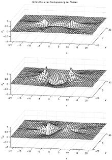
Griffith crack under compressive stress on the crack flanks

In the case of a crack with normal loading in the y-direction on the crack flanks (internal pressure), the complex stress functions result ${\displaystyle {\sigma }^{0}}$

${\displaystyle {\begin{array}{ll}\Phi (z)&={\frac {-{\sigma }^{0}a}{2}}\zeta \\\Psi (z)&=-{\sigma }^{0}a{\frac {\zeta }{1-\zeta ^{2}}}\end{array}}}$

and the tensions

${\displaystyle {\begin{array}{ll}\sigma _{xx}(z)&=2{\sigma }^{0}\Re \left\{{\frac {\zeta ^{2}}{1-\zeta ^{2}}}-{\frac {2\zeta ^{3}}{{(1-\zeta ^{2})}^{3}}}{\frac {z-{\bar {z}}}{a}}\right\}\\\sigma _{yy}(z)&=2{\sigma }^{0}\Re \left\{{\frac {\zeta ^{2}}{1-\zeta ^{2}}}+{\frac {2\zeta ^{3}}{{(1-\zeta ^{2})}^{3}}}{\frac {z-{\bar {z}}}{a}}\right\}\\\tau _{xy}(z)&=4{\sigma }^{0}\Im \left\{{\frac {\zeta ^{3}}{{(1-\zeta ^{2})}^{3}}}{\frac {z-{\bar {z}}}{a}}\right\}\end{array}}}$.

When approaching the crack tips, they grow across all boundaries: there is a singularity here. In the picture, the voltage peaks are only shown up to a certain maximum value, hence the plateaus. ${\displaystyle \zeta \rightarrow {\pm }1}$

Shear load on the crack flanks

Griffith crack with shear stress on the crack flanks

In the case of a crack with shear loads on the crack flanks, the complex stress functions arise ${\displaystyle \tau ^{0}}$

${\displaystyle {\begin{array}{ll}\Phi (z)&={\frac {\mathrm {i} \tau ^{0}a}{2}}\zeta \\\Psi (z)&=\mathrm {i} \tau ^{0}a{\frac {\zeta ^{3}}{1-\zeta ^{2}}}\end{array}}}$

and the tensions

${\displaystyle {\begin{array}{ll}\sigma _{xx}(z)&=4\tau ^{0}\Im \left\{{\frac {\zeta ^{2}}{1-\zeta ^{2}}}-{\frac {\zeta ^{3}}{{(1-\zeta ^{2})}^{3}}}{\frac {z-{\bar {z}}}{a}}\right\}\\\sigma _{yy}(z)&=4\tau ^{0}\Im \left\{{\frac {\zeta ^{3}}{{(1-\zeta ^{2})}^{3}}}{\frac {z-{\bar {z}}}{a}}\right\}\\\tau _{xy}(z)&=2\tau ^{0}\Re \left\{{\frac {\zeta ^{2}}{1-\zeta ^{2}}}-{\frac {2\zeta ^{3}}{{(1-\zeta ^{2})}^{3}}}{\frac {z-{\bar {z}}}{a}}\right\}\end{array}}}$.

When approaching the crack tips, they grow across all boundaries: there is a singularity here. In the picture, the voltage peaks are only shown up to a certain maximum value, hence the plateaus. ${\displaystyle \zeta \rightarrow {\pm }1}$

See also

• Technical mechanics
• Continuum mechanics
• Geometric linearization
• Linear-elastic fracture mechanics deals with cracks in elastic media.

Footnotes

1. ↑ Faal, RT, and SJ Fariborz. " Stress analysis of orthotropic planes weakened by cracks. " Applied mathematical modeling 31.6 (2007): 1133-1148.
2. ↑ Hufenbach, Ing W., and Ing AS Herrmann. " Calculation of the stress and displacement field of anisotropic disks with an elliptical section. " Ingenieur-Archiv 60.8 (1990): 507-517.
3. ↑ R. Greeve (2003), pp 128ff
4. ↑ In HG Hahn 1976, the stress functions for a Griffith crack under uniaxial tensile load at an angle to the crack are included ${\displaystyle {\sigma }^{0}}$ ${\displaystyle \varphi =\beta }$

   ${\displaystyle {\begin{array}{ll}\Phi (z)&={\frac {{\sigma }^{0}a}{8}}\left({\frac {1}{\zeta }}+\left(2e^{2\mathrm {i} \beta }-1\right)\zeta \right)\\\Psi (z)&={\frac {-{\sigma }^{0}a}{4}}\left({\frac {e^{-2\mathrm {i} \beta }}{\zeta }}+{\frac {\left(2-e^{2\mathrm {i} \beta }\right)\zeta -e^{2\mathrm {i} \beta }\zeta ^{3}}{1-\zeta ^{2}}}\right)\end{array}}}$

   specified. Superposition with the homogeneous stress state leads to the functions shown here. ${\displaystyle F_{\beta }}$

literature

• H. Parisch: Solid Continuum Mechanics . Teubner, 2003, ISBN 3-519-00434-8 .
• HG Hahn: fracture mechanics , Teubner study books: mechanics, BG Teubner Stuttgart 1976.
• NI Musschelischwili: Some basic tasks on the mathematical theory of elasticity. C. Hanser, 1971.
• W. Becker, D. Gross: Mechanics of elastic bodies and structures . Springer, 2002. ISBN 3-540-43511-5 , limited preview in the Google book search
• Gross, Th. Seelig: fracture mechanics . Springer, 2001. ISBN 3-540-42203-X .
• H. Grote, J. Feldhusen (Hrsg.): Dubbel paperback for mechanical engineering. Springer, 2011. ISBN 978-3-642-17305-9 , limited preview in the Google book search
• IS Sokolnikoff: Mathematical Theory of Elasticity , Robert E. Krieger Publishing Company, Malabar, Florida 1983.