Rivers and cuts in networks

Flows and cuts in networks are structures of graph theory that find diverse applications.

Definitions, important terms and properties

network

A network (engl. Network ) consists of a directed graph with two excellent node (engl. Vertex / vertices ), a source (engl. Source ) and a sink (Engl. Target ) from , and a capacity function that each edge of a non-negative Allocates capacity . If the capacity function only has integer values, there is a maximum flow function (see definition below), which also only has integer values. ${\displaystyle N=(G,u,s,t)}$ ${\displaystyle G=(V,E)}$ ${\displaystyle s}$ ${\displaystyle t}$ ${\displaystyle V}$ ${\displaystyle u\colon E\rightarrow \mathbb {R} _{+}}$ ${\displaystyle e\in E}$ ${\displaystyle e\mapsto u(e)}$

flow

• 

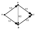
  Example of a river . The occupancy is together with the capacity on the individual edges. The value of the - flow is 2. ${\displaystyle s}$ ${\displaystyle t}$

• 

  Example of a residual network . On the path , , , can the flow to the value 2 augment . ${\displaystyle s}$ ${\displaystyle a}$ ${\displaystyle b}$ ${\displaystyle t}$

A flow is a function that assigns a non-negative flow value to each edge in the network . The following condition must be met: ${\displaystyle f\colon E\rightarrow \mathbb {R} _{+}}$ ${\displaystyle e\in E}$ ${\displaystyle f(e)\in \mathbb {R} _{+}}$

Capacity conformity:

The flow value on an edge is at most as large as the capacity of the edge, that is, the following applies:

${\displaystyle \forall e\in E:f(e)\leq u(e)}$.

If the following condition is also met, the flow is called - -flow: ${\displaystyle s}$ ${\displaystyle t}$

River maintenance:

Apart from the source s and the sink t , exactly as much must flow into each node as flows out, that is:

${\displaystyle \forall v\in V\setminus \{s,t\}:\sum _{e\in \operatorname {\delta ^{-}} (v)}f(e)=\sum _{e\in \operatorname {\delta ^{+}} (v)}f(e)}$

It is

${\displaystyle \operatorname {\delta ^{-}} (v){\overset {\underset {\mathrm {def} }{}}{=}}\{e=(x,v)\in E\mid x\in V\}}$

the amount of into and ${\displaystyle v}$

${\displaystyle \operatorname {\delta ^{+}} (v){\overset {\underset {\mathrm {def} }{}}{=}}\{e=(v,x)\in E\mid x\in V\}}$

the amount of edges leading out. ${\displaystyle v}$

If river conservation also applies in and , there is a current or circulation . One can show that incidence vectors correspond to a circulation if they lie in the cycle space of . ${\displaystyle s}$ ${\displaystyle t}$ ${\displaystyle Z(G)}$ ${\displaystyle G}$

value

The value of a - -flow is the excess in the node or the amount of the excess in the node . ${\displaystyle s}$ ${\displaystyle t}$ ${\displaystyle f}$ ${\displaystyle t}$ ${\displaystyle s}$

In formulas:

${\displaystyle |f|=\sum _{e\in \operatorname {\delta ^{+}} (s)}f(e)-\sum _{e\in \operatorname {\delta ^{-}} (s)}f(e)}$, where denotes the source of the network. ${\displaystyle s}$

For all - flows the excess is zero except for all nodes. It is also in zero for all circulations . ${\displaystyle s}$ ${\displaystyle t}$ ${\displaystyle s,t}$ ${\displaystyle s,t}$

excess

The excess of a node , also called net flow or surplus , is the difference between the sum of the flow values ​​of the incoming edges and the sum of the flow values ​​of the outgoing edges. ${\displaystyle \operatorname {ex} (v)}$ ${\displaystyle v}$

${\displaystyle \operatorname {ex} (v){\overset {\underset {\mathrm {def} }{}}{=}}\sum _{e\in \operatorname {\delta ^{-}} (v)}f(e)-\sum _{e\in \operatorname {\delta ^{+}} (v)}f(e)}$

Example of a cut . The capacity of the cut is ${\displaystyle {\begin{aligned}&\quad \ u((s,b))\\&+u((a,b))\\&+u((a,t))\\&=1+2+1=4\\\end{aligned}}}$

cut

A proper subset of the nodes in a network, but not including, it's called a - fraction . A cut is often understood to be the set of all edges that run between the partitions and . The capacity of a cut is the sum of the capacities of the edges running from to . ${\displaystyle S}$ ${\displaystyle s}$ ${\displaystyle t}$ ${\displaystyle s}$ ${\displaystyle t}$ ${\displaystyle S}$ ${\displaystyle V\setminus S}$ ${\displaystyle S}$ ${\displaystyle V\setminus S}$

Sections give an upper bound on the value of the - flows. The Max-Flow-Min-Cut-Theorem states that, conversely, flow values ​​are also a lower bound for cutting capacities. So both concepts correspond in a natural way. ${\displaystyle s}$ ${\displaystyle t}$

Residual network

The residual network , or residual network , to the flow with residual graphs and residual capacities shows the remaining capacities of the network. The residual graph has the same set of nodes as and consists of the unused edges supplemented by back edges: For each edge with contains a back edge . The residual capacities indicate for an edge by how much the flow on it can still be increased, and for a rear edge by how much the flow on the associated trailing edge can be reduced. So: ${\displaystyle N_{f}}$ ${\displaystyle f}$ ${\displaystyle G_{f}}$ ${\displaystyle u_{f}}$ ${\displaystyle G_{f}}$ ${\displaystyle G}$ ${\displaystyle f}$ ${\displaystyle e=(v,w)\in E}$ ${\displaystyle f(e)>0}$ ${\displaystyle E_{f}}$ ${\displaystyle {\overleftarrow {e}}=(w,v)}$ ${\displaystyle u_{f}(e)}$ ${\displaystyle e\in E}$ ${\displaystyle {\overleftarrow {e}}}$

${\displaystyle \forall e\in E:u_{f}(e)=u(e)-f(e)}$if ${\displaystyle f(e)<u(e)}$

${\displaystyle \forall {\overleftarrow {e}}\in E_{f}\setminus E:u_{f}({\overleftarrow {e}})=f(e)}$

Algorithmic construction of a residual network

Initialisiere  ${\displaystyle E_{f}=\emptyset }$;  ${\displaystyle u_{f}\equiv u}$;
1. Für alle Kanten  ${\displaystyle e\in E}$
2.    if( ${\displaystyle f(e)>0}$)
3.       Füge  ${\displaystyle {\overleftarrow {e}}}$ in  ${\displaystyle E_{f}}$ ein
4.       Setze  ${\displaystyle u_{f}({\overleftarrow {e}}):=\!\,\!\,f(e)}$
5.    if( ${\displaystyle f(e)<u(e)}$)
6.       Füge  ${\displaystyle e}$ in  ${\displaystyle E_{f}}$ ein
7.       Setze  ${\displaystyle u_{f}(e):=\!\,\!\,u(e)-f(e)}$
8. gib aus  ${\displaystyle N_{f}=(V,E_{f},u_{f},s,t)}$

Layer network

The level of a node is the number of edges of a shortest path from to in the residual network to the river . The -th level of a graph the set of all nodes with Level so . An edge with a flow value is called useful from to if . If true , it is called useful from to . An edge is called useful from a set if it is useful from an element of the set to an element outside the set. Similarly, one explains useful in a lot . The layer network or level network to the river is a subgraph of with ${\displaystyle \operatorname {level} (v){\overset {\underset {\mathrm {def} }{}}{=}}\delta _{f}(s,v)}$ ${\displaystyle s}$ ${\displaystyle v}$ ${\displaystyle f}$ ${\displaystyle i}$ ${\displaystyle i}$ ${\displaystyle V_{i}{\overset {\underset {\mathrm {def} }{}}{=}}\{v\in V\mid \operatorname {level} (v)=i\}}$ ${\displaystyle e=(w,v)}$ ${\displaystyle f(e)}$ ${\displaystyle w}$ ${\displaystyle v}$ ${\displaystyle f(e)<u(e)}$ ${\displaystyle f(e)>0}$ ${\displaystyle v}$ ${\displaystyle w}$ ${\displaystyle {\tilde {N_{f}}}}$ ${\displaystyle f}$ ${\displaystyle G}$

1. ${\displaystyle {\tilde {V_{f}}}{\overset {\underset {\mathrm {def} }{}}{=}}V}$
2. ${\displaystyle {\tilde {E_{f}}}{\overset {\underset {\mathrm {def} }{}}{=}}\{e=(w,v)\in E_{f}\mid \operatorname {level} (w)=\operatorname {level} (v)-1\}}$

The stratified and residual network can be calculated in linear time.

Special paths and rivers

An xy-way or path is a sequence of edges, with the starting node of each edge being the terminal node of its predecessor. The length of a path , also is the number of edges in the way. ${\displaystyle W(x,y)}$ ${\displaystyle \delta _{W}(x,y)}$ ${\displaystyle dist_{W}(x,y)}$

The distance between and is the length of a shortest path, if one exists, and "infinite" if not. A path in the residual network is called an augmenting path ; the terms improving route or enhancing route are also in use. Every - -flow can be broken down into rivers on - -ways and into circles. Exactly when there is no augmenting path to a - - flow in a network , the flow has maximum value. The algorithm of Ford and Fulkerson and the algorithm of Edmonds and Karp exploit this fact . ${\displaystyle x}$ ${\displaystyle y}$ ${\displaystyle s}$ ${\displaystyle t}$ ${\displaystyle s}$ ${\displaystyle t}$ ${\displaystyle s}$ ${\displaystyle t}$

A flow in a network is blocking if every - path in an edge block , or saturated , is d. H. . ${\displaystyle f}$ ${\displaystyle (G,u,s,t)}$ ${\displaystyle s}$ ${\displaystyle t}$ ${\displaystyle G}$ ${\displaystyle e}$ ${\displaystyle f(e)=u(e)}$

Push operation

${\displaystyle \operatorname {PUSH} (v,w)}$ -> Voraussetzungen: ${\displaystyle v\in V}$ hat Exzess, ${\displaystyle u_{f}(v,w)>0}$ und ${\displaystyle \operatorname {h} (v)=\operatorname {h} (w)+1}$ -> Beschreibung: Schiebe ${\displaystyle d_{f}(v,w){\overset {\underset {\mathrm {def} }{}}{=}}min\{\operatorname {ex} (v),u_{f}(v,w)\}}$ Einheiten Fluss von ${\displaystyle v}$ nach ${\displaystyle w}$ 1. ${\displaystyle d_{f}(v,w)\leftarrow min\{\operatorname {ex} (v),u_{f}(v,w)\}}$ 2. ${\displaystyle f(v,w)\leftarrow f(v,w)+d_{f}(v,w)}$ 3. ${\displaystyle f(w,v)\leftarrow -f(v,w)}$ 4. ${\displaystyle \operatorname {ex} (v)\leftarrow \operatorname {ex} (v)-d_{f}(v,w)}$ 5. ${\displaystyle \operatorname {ex} (w)\leftarrow \operatorname {ex} (w)+d_{f}(v,w)}$

Lift operation

${\displaystyle \operatorname {LIFT} (v)}$ Voraussetzungen: ${\displaystyle v\in V}$ hat Exzess und es gilt für beliebige ${\displaystyle w\in V}$: ${\displaystyle (v,w)\in E_{f}\Rightarrow \operatorname {h} (v)\leq \operatorname {h} (w)}$ Beschreibung: inkrementiere die Höhe von ${\displaystyle v}$ 1. ${\displaystyle \operatorname {h} (v)\leftarrow 1+min\{\operatorname {h} (w)\mid (v,w)\in E_{f}\}}$

Pre-flows

${\displaystyle s}$- - Präflüsse , or Vorflüsse , (Engl. Preflow ) are a generalization of - fluxes. This term is only relevant for more complex (and much more efficient) flow algorithms. ${\displaystyle t}$ ${\displaystyle s}$ ${\displaystyle t}$

A - pre-flow is a function with capacity conformity as above and the following weakening of the flow maintenance: ${\displaystyle s}$ ${\displaystyle t}$ ${\displaystyle f\colon A\rightarrow \mathbb {R} _{+}}$

${\displaystyle \forall u\in V\setminus \{s\}:\operatorname {ex} (u)\geq 0}$

This means that more flow may only leave the node than reaches it. A - pre-flow has excess in a node, or overflow , if its excess (as above) is really greater than zero. The residual network is formed in the same way as above. ${\displaystyle s}$ ${\displaystyle s}$ ${\displaystyle t}$

The height function or distance marking in a network with - - Preflux is an illustration with , and for all edges . ${\displaystyle s}$ ${\displaystyle t}$ ${\displaystyle f}$ ${\displaystyle \operatorname {h} \colon V\rightarrow \mathbb {N} _{0}}$ ${\displaystyle \operatorname {h} (s)=|V|}$ ${\displaystyle \operatorname {h} (t)=0}$ ${\displaystyle \operatorname {h} (v)\leq \operatorname {h} (w)+1}$ ${\displaystyle e=(v,w)\in E_{f}}$

Furthermore, the push and lift operations are explained algorithmically, as described on the right. With these means one can design and study preflow push algorithms , such as the Goldberg-Tarjan algorithm (after Andrew Goldberg and Robert Tarjan ). With these algorithms, the data structures cannot be interpreted as - -flow while the algorithm is running . Goldberg and Tarjan's method initializes a pre-flow and terminates if certain manipulations of the structure produce a - -flow. This is always the case there after a finite number of steps and this - -flow is then always at its maximum. ${\displaystyle s}$ ${\displaystyle t}$ ${\displaystyle s}$ ${\displaystyle t}$ ${\displaystyle s}$ ${\displaystyle t}$

Algorithms

The algorithm by Ford and Fulkerson gradually searches for augmenting paths, i.e. paths in the residual network, and increases along them. This procedure works exactly when this algorithm terminates, i.e. when it comes into the situation that there are actually no more augmenting paths. Then one can consider the maximum number of nodes that can be reached in the residual network. This defines a - -cut, the capacity of which equals the flow value. ${\displaystyle s}$ ${\displaystyle s}$ ${\displaystyle t}$

To secure the termination, however, one can use an argument about the algebraic structure of the capacitance values. If they are nonnegative integers , the value of a maximum - -flow is an integer. In addition, there is at least one maximum st-flow which only assumes integer values ​​edge-wise. This need not be the case for every maximum st flow. Because each augmentation along a - path increases the value of the - flow by an integer step, i.e. by at least 1, the termination is ensured after a finite number of steps in the case. An upper limit on the running time of the algorithm can then depend on the values ​​of the capacities. The running time can then be arbitrarily large in relation to the number of nodes and edges, depending on the capacities on the edges. If the capacities are nonnegative rational numbers, the Ford-Fulkerson algorithm also terminates because the network is then algorithmically equivalent to a network in which the capacities are multiplied by the main denominator, i.e. only integer capacities occur. In the case of real, irrational capacities, however, the algorithm does not have to terminate and does not even have to converge to a maximum - -flow. ${\displaystyle s}$ ${\displaystyle t}$ ${\displaystyle s}$ ${\displaystyle t}$ ${\displaystyle s}$ ${\displaystyle t}$ ${\displaystyle s}$ ${\displaystyle t}$

The Edmonds-Karp algorithm is a further development of the Ford and Fulkerson method: It works completely analogously, but seeks augmenting paths that are minimal in terms of the number of edges. This works with a breadth-first search in linear time. The Edmonds-Karp algorithm also terminates with any real edge capacities. In addition, its running time , i.e. generally in terms of magnitude, is significantly better than the Ford-Fulkerson algorithm. ${\displaystyle {\mathcal {O}}(|V|\cdot |E|^{2})}$

The Dinic algorithm is based on another observation. If you look for an augmenting path in the residual network, it can happen that you come to a dead end, i.e. to a node from which it is not at all accessible. The idea is to layer the network, i.e. to combine it into groups that are at the same distance , i.e. such dead ends are eliminated. In this layer network , one then takes advantage of the fact that a search not only yields a route, but also a route tree without any additional effort . You can then send flow along this tree and block the network. All of this is fundamentally possible with a modified depth-first search. In the next iteration, you then have the situation that you need at least one more layer because the old layer is blocked. The argument to limit the number of layers to a maximum of pieces provides a limit to the number of so-called phase runs of the algorithm, i.e. the number of loop iterations. This results in a running time of . ${\displaystyle t}$ ${\displaystyle s}$ ${\displaystyle {\mathcal {O}}(|V|\cdot |E|)}$ ${\displaystyle |V|-1}$ ${\displaystyle {\mathcal {O}}(|V|^{2}\cdot |E|)}$

The following table gives an overview of the developed flow algorithms and their runtimes:

Max-Flow algorithms after publication

Formulations as a linear program

The problem of maximizing the flow value can also be described as a linear optimization problem . For example, if you choose a variable for each edge that measures the flow on the edge, you get the following program: ${\displaystyle |f|}$ ${\displaystyle x_{e}}$ ${\displaystyle e\in E}$ ${\displaystyle f(e)}$

${\displaystyle {\begin{aligned}\max &\sum _{e\in \operatorname {\delta ^{+}} (s)}x_{e}-\sum _{e\in \operatorname {\delta ^{-}} (s)}x_{e}\\{\text{so dass }}&\forall v\in V\setminus \{s,t\}\colon \;\sum _{e\in \operatorname {\delta ^{-}} (v)}x_{e}=\sum _{e\in \operatorname {\delta ^{+}} (v)}x_{e}\\&\forall \;e\in E\colon \;x_{e}\geq 0\;\;\\&\forall \;e\in E\colon \;x_{e}\leq u_{e}\\\end{aligned}}}$

An alternative formulation is obtained if one introduces a variable for each - path , which describes the flow on the corresponding path. The result is the following program: ${\displaystyle s}$ ${\displaystyle t}$ ${\displaystyle P}$ ${\displaystyle x_{P}}$

${\displaystyle {\begin{aligned}\max &\sum _{P\in {\mathcal {P}}_{(s,t)}}x_{P}\\{\text{so dass }}&\forall \;e\in E\colon \;\sum _{P\in {\mathcal {P}}_{(s,t)},\;e\in P}x_{P}\leq u_{e}\\&\forall \;P\in {\mathcal {P}}_{(s,t)}\colon \;x_{P}\geq 0\end{aligned}}}$

Here referred to the set of all paths from to . ${\displaystyle {\mathcal {P}}_{(s,t)}}$ ${\displaystyle s}$ ${\displaystyle t}$

The second formulation seems unfavorable at first, since the number of - paths generally increases exponentially with the number of nodes and edges. Nevertheless, this formulation can be solved efficiently by generating columns, i.e. in polynomial time. ${\displaystyle s}$ ${\displaystyle t}$

The two formulations also have the property that the matrices that describe the secondary conditions are totally unimodular . This means that every optimal solution of the two programs is an integer, provided that the capacities are integers. ${\displaystyle u_{e}}$

It is also instructive to look at the dualizations of the above programs. For the path-based formulation, the dual program is given, for example, by:

${\displaystyle {\begin{aligned}\min &\sum _{e\in E}u_{e}y_{e}\\{\text{so dass }}&\forall \;P\in {\mathcal {P}}_{(s,t)}\colon \;\sum _{e\in P}y_{e}\geq 1\\&\forall \;e\in E\colon \;y_{e}\geq 0\end{aligned}}}$

The dual program is also totally unimodular. This implies that the optimal solution of the dual program is a vector with entries. For every feasible -vector , the set also corresponds to a - -cut. The optimal solution of the dual program thus corresponds to a - -cut of minimum capacity. From this the Max-Flow-Min-Cut theorem follows from the strong duality principle of linear optimization . ${\displaystyle 0/1}$ ${\displaystyle |E|}$ ${\displaystyle 0/1}$ ${\displaystyle y}$ ${\displaystyle \{e\in E\,:\,y_{e}=1\}}$ ${\displaystyle s}$ ${\displaystyle t}$ ${\displaystyle s}$ ${\displaystyle t}$

Generalizations

There are some key generalizations about the problem. First, instead of rivers between a source or sink , one can consider rivers between areas. To do this, you give yourself a certain number of suppliers and a number of recipients , as well as a graph and capacities. The problem is not heavier than Max-flow and can either forward and downstream connection of additional nodes or through the transition to the quotient graph on Max-Flow reduced to. ${\displaystyle S}$ ${\displaystyle T}$ ${\displaystyle G/_{S\cup T}}$

On the other hand, one can extend the validity of the capacities assigned to the edges to a certain neighborhood of the edge, where for a fixed a- neighborhood is the set of nodes and edges that are elements away from the edge. The special case corresponds to the maximum flow problem. The case corresponds to the maximum flow problem with node capacities. This can be reduced to Max-Flow by replacing the nodes with something like the one in the picture. The number of edges is not constantly changed, so the complexity of the problem increases. However, there are solutions for Max-Flow, the complexity of which strictly depends on the nodes, the number of which changes by a constant factor of 2 at most. ${\displaystyle d\in \mathbb {N} }$ ${\displaystyle d}$ ${\displaystyle d}$ ${\displaystyle d=0}$ ${\displaystyle d=1}$

In this case , one can prove that the problem is NP-complete and therefore presumably cannot be solved in polynomial time (unless ). A polynomial algorithm was found for this case. ${\displaystyle d\geq 3}$ ${\displaystyle P=NP}$ ${\displaystyle d=2}$

application

Practical applications

This last generalization is motivated by problems with the cabling of VLSI chips , where it is difficult to put more cables in a certain vicinity of laid cables.

The flow theory has historically developed on the basis of problems from application. In general, the assumption was made that a fluid , i.e. an object that can be broken down into any number of sub-objects, is spatially displaced through a world in various ways - for example electrical energy from a source to a place of demand via a power network, or data from a transmitter via a data network to a recipient. You can also model abstract objects such as “know each other”. Using maximum flows in a social network, one can then obtain a measure of how strongly two (sets of) people are networked with one another.

Bipartite graph with the node sets A (red) and B (green) and the added source s and sink t

Theoretical applications

The flow theory has an obvious and natural application in the transversal theory, which can be embedded in the theory of flows in a very natural way. Ford formulated a comprehensive approach to this in a standard work in 1962.

Many combinatorial problems on graphs, such as bipartite matchings , can easily be converted into a suitable flow problem (see picture) and quickly solved there. Another application is the efficient determination of the node connection number , edge connection number or arc connection number . By Lemma Tutte (after William Thomas Tutte ) also extended applications flow theory (so-called gruppenwertigen rivers) and Färbbarkeitsaussagen significantly. Some of his assumptions about the existence of k-flows in planar graphs have strong theoretical implications.

literature

• Bernhard Korte , Jens Vygen : Combinatorial Optimization: Theory and Algorithms . Translated from the English by Rabe von Randow. Springer-Verlag, Berlin Heidelberg 2008, ISBN 978-3-540-76918-7
• Alexander Schrijver : Combinatorial Optimization: Polyhedra and Efficiency , Springer-Verlag, 2003, ISBN 3-540-44389-4
• Thomas H. Cormen, Charles E. Leiserson , Ronald L. Rivest , Clifford Stein: Introduction to Algorithms . 2nd Edition. MIT Press, Cambridge (Massachusetts) 2001, ISBN 0-262-03293-7 .
• Lester Randolph Ford junior , Delbert Ray Fulkerson : Flows in Networks . 1962, ISBN 0-691-07962-5 , ISBN 978-0-691-07962-2 .