Perceptron

Simple two-ply feed-forward perceptron with

five input neurons,

three hidden neurons and

an output neuron, as well

two bias neurons

The Perceptron (after English. Perception , "perception") is a simplified artificial neural network , first described by Frank Rosenblatt was the market in 1958. In the basic version (simple perceptron) it consists of a single artificial neuron with adjustable weightings and a threshold value. This term, various combinations of the original model are now understood distinction is made between single-layer and multi-layer (Engl. Perzeptren multi-layer perceptron MLP) distinguished. Perceptron networks convert an input vector into an output vector and thus represent a simple associative memory.

history

Simple perceptron that implements a logical OR.

Input neurons

Output neuron

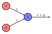
In 1943 the mathematicians Warren McCulloch and Walter Pitts introduced the “neuron” as a logical threshold element with several inputs and a single output in computer science. As a Boolean variable, it could assume the states true and false and "fired" (= true ) when the sum of the input signals exceeded a threshold value. This corresponded to the neurobiological analogy of an action potential that a nerve cell emits when its membrane potential changes critically. McCulloch and Pitts showed that any simple propositional function (AND, OR, NOT) can be described by a suitable combination of several such neurons.

In 1949, the psychologist Donald O. Hebb hypothesized that learning is based on the fact that the activating or inhibiting effect of a synapse can be calculated as the product of pre- and postsynaptic activity . There are indications that long-term potentiation and so-called spike-timing dependent plasticity (STDP) are the biological correlates of Hebb's postulate . Convincing evidence for this thesis is still pending.

In 1958 Frank Rosenblatt finally published the perceptron model, which to this day represents the basis of artificial neural networks.

Single layer perceptron

In the single-layer perceptron, there is only a single layer of artificial neurons, which also represents the output vector. Each neuron is represented by a neuron function and receives the entire input vector as a parameter. The processing is very similar to what is known as Hebb's learning rule for natural neurons. However, the activation factor of this rule is replaced by a difference between the setpoint and the actual value. Since Hebb's learning rule relates to the weighting of the individual input values, a perceptron is learned by adapting the weighting of each neuron. Once the weights have been learned, a perceptron is also able to classify input vectors that differ slightly from the originally learned vector. This is precisely what makes the perceptron capable of classification, from which it owes its name.

Calculation of the output values

With a bias , the inputs and the weights of the output values calculated for ${\displaystyle b}$ ${\displaystyle x_{i}}$ ${\displaystyle w_{ij}}$ ${\displaystyle o_{j}}$

${\displaystyle o_{j}={\begin{cases}1&\sum _{i}w_{ij}x_{i}+b>0\\0&{\text{ansonsten}}\end{cases}}}$.

Remarks

• The bias is provided as a threshold value (engl. Threshold ) is set with a negative sign. ${\displaystyle b}$ ${\displaystyle \theta }$
• If the threshold value is used instead , the first condition results and the corresponding sign also changes for the associated function term. ${\displaystyle \theta }$ ${\displaystyle \sum _{i}w_{ij}x_{i}-\theta \neq 0}$

Perceptron learning rule

There are different versions of the learning rule to address the different definitions of the perceptron. The learning rule is specified here for a perceptron with binary input and output values. This rule only converges if the training data set can be linearly separated , see below under "Variants" .

The learning rule of the perceptron is based on the following considerations:

1. If the output of a neuron is 1 (or 0) and should assume the value 1 (or 0), the weightings are not changed.
2. If the output is 0, but should assume the value 1, then the weights are incremented .
3. If the output is 1, but should assume the value 0, then the weights are decremented .

Mathematically, the matter is expressed as follows:

${\displaystyle w_{ij}^{\mathrm {neu} }=w_{ij}^{\mathrm {alt} }+\Delta w_{ij}}$,

${\displaystyle \Delta w_{ij}=\alpha \cdot (t_{j}-o_{j})\cdot x_{i}}$.

It is

${\displaystyle \Delta w_{ij}}$the change in weight for the connection between the input cell and output cell , ${\displaystyle w_{ij}}$ ${\displaystyle i}$ ${\displaystyle j}$

${\displaystyle t_{j}}$the desired output of the neuron , ${\displaystyle j}$

${\displaystyle o_{j}}$ the actual output,

${\displaystyle x_{i}}$the input of the neuron and ${\displaystyle i}$

${\displaystyle \alpha >0}$ the learning rate.

A weight update in step then proceeds as follows: ${\displaystyle k}$

1. ${\displaystyle w_{ij}(k+1)=w_{ij}(k)}$ with correct output,
2. ${\displaystyle w_{ij}(k+1)=w_{ij}(k)+\alpha x_{i}}$ for output 0 and desired output 1 and
3. ${\displaystyle w_{ij}(k+1)=w_{ij}(k)-\alpha x_{i}}$ for output 1 and desired output 0.

Rosenblatt was able to prove in the convergence theorem that all solutions that a perceptron can represent can be learned with the specified learning procedure.

XOR problem

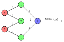
Frank Rosenblatt showed that a simple perceptron with two input values ​​and a single output neuron can be used to represent the simple logical operators AND, OR and NOT. However, in 1969, Marvin Minsky and Seymour Papert showed that a single-layer perceptron cannot resolve the XOR operator (problem of linear separability ). This led to a standstill in the research of artificial neural networks.

The discussion, which was in part extremely polemical in this context , was ultimately a dispute over the direction of the representatives of symbolic artificial intelligence and the “connectionists” over research funding. Frank Rosenblatt had shown that logical operators such as XOR (identical to the composition OR but NOT AND) can be described using a multi-layer perceptron, but he died too early to defend himself against the attacks of his AI colleagues.

Variants of the perceptron learning rule

The standard learning rule given above only converges if the training data set can be linearly separated . If this is not the case, the standard learning rule will not generate an approximate solution (for example a solution with as few incorrectly assigned data as possible). Instead, the learning process will fail completely.

Since linear separability of the training data set is often not known before training begins, variants of the training algorithm should therefore be used that are robust in the sense that they converge to an approximate solution in the non-linearly separable case.

One such robust method is the Maxover algorithm. In the linearly separable case, it solves the training problem completely, even under further optimization conditions such as maximum stability (maximum distance between the data with output 0 and 1). In the non-linearly separable case, it generates a solution with a few incorrectly assigned data. In both cases there is a gradual approach to the solution in the course of the learning process. The algorithm converges to a globally optimal solution in the linearly separable case, or to a locally optimal solution in the non-linearly separable case.

The pocket algorithm learns with a standard perceptron learning rule. He keeps the solution that has so far produced the fewest incorrectly assigned data in his "pocket" and outputs it as an approximate solution. In the linearly separable case, this algorithm learns completely. In the non-linearly separable case, use is made of the fact that the standard perceptron learning rule produces random solutions, among which such approximate solutions appear stochastically. The pocket algorithm therefore has disadvantages: On the one hand, there is no gradual approach to the solution, but stochastic jumps are used. Since these occur at unpredictable times in the learning process, there is no certainty as to how close the algorithm has come to an optimal solution after a certain number of learning steps. On the other hand, the total number of correctly assigned data must be determined in each learning step. The algorithm does not work locally, as is typical for neural networks.

If the linear separability of the training data set is known , different variants of the standard perceptron learning rule can be used. The "perceptron of optimal stability" (maximum distance between the data with output "0" and "1") can be generated with the min-over algorithm (Krauth and Mezard, 1987). A particularly fast algorithm based on quadratic optimization is the AdaTron (Anlauf and Biehl, 1989). Optimal stability, together with the kernel trick, are the conceptual requirements of the support vector machine .

The perceptron as a linear classifier

Beyond all (pseudo-) biological analogies, a single-layer perceptron is ultimately nothing more than a linear classifier of form (linear discriminant function , multiple linear regression ). In the nomenclature of artificial neural networks, up to are referred to as weights and up to as input signals, whereby the latter can only assume values ​​of 1 or 0 (“true” or “false”). If the total exceeds a threshold value, the assignment of the class being searched for is set to “true” or 1, otherwise to “false” or 0. ${\displaystyle x=a_{1}y_{1}+a_{2}y_{2}+\cdots +a_{n}y_{n}}$ ${\displaystyle a_{1}}$ ${\displaystyle a_{n}}$ ${\displaystyle y_{1}}$ ${\displaystyle y_{n}}$ ${\displaystyle x}$

Multi-layer perceptron

Two-layer perceptron for calculating the XOR function

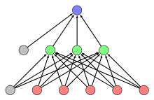
The limitation of the single-layer perceptron could later be solved with the multi-layer perceptron, in which there is at least one additional layer of hidden neurons in addition to the output layer . If the outputs are only linked to inputs of a subsequent layer, so that the flow of information only runs in one direction, we speak of feed-forward networks. The following topologies have proven themselves:

• Fully connected: The neurons of one layer are connected to all neurons of the immediately following layer.
• Short cuts: Some neurons are not only connected to all neurons in the next layer, but also to other neurons in the next but one layer.

If there are neurons in the network whose outputs are connected to neurons of the same or a previous layer, it is a recurrent neural network .

Multi-layer perceptrons require more complex learning rules than single-layer perceptrons. Backpropagation is a possible algorithm for supervised learning .

The expansion of these network topologies to include additional hidden layers and the introduction of other architectures (for example recurrent neural networks ), which are also mostly trained using backpropagation , is now summarized under the keyword deep learning .

literature

• Rosenblatt, Frank (1958): The perceptron: a probabilistic model for information storage and organization in the brain . Psychological Reviews 65 (1958) 386-408
• ML Minsky and SA Papert, Perceptrons. 2nd Edition, MIT-Press 1988, ISBN 0-262-63111-3

Web links

• Blog post about the perceptron in German with examples and code
• Multi-part tutorial series in simple language about the perceptron

Individual evidence

1. ^ A logical calculus of the ideas immanent in nervous activity . WS McCulloch, W Pitts. Bull Math. Biophys., 5, 115-133, 1943.
2. ^ Organization of Behavior . D Hebb. Wiley. New York. 1949.
3. ↑ The perceptron - a probabilistic model for information storage and organization in the brain . F rose petal. Psychological Review 65, 1958.
4. ↑ Michael Nielsen: Chapter 1: Using neural nets to recognize handwritten digits. Section: Perceptrons. Accessed August 9, 2019 . 
5. ^ Andreas Wendemuth: Learning the Unlearnable . In: Journal of Physics A: Math. Gen. 28 . 1995, p. 5423–5436 ( PDF ( memento of March 5, 2016 in the Internet Archive ) [accessed on March 14, 2016]).
6. ^ SI Gallant. Perceptron-based learning algorithms. IEEE Transactions on Neural Networks, vol. 1, no. 2, pp. 179-191 (1990)
7. ↑ W. Krauth and M. Mezard. Learning algorithms with optimal stability in neural networks. J. of Physics A: Math. Gen. 20: L745-L752 (1987)
8. ^ JK Anlauf and M. Biehl. The AdaTron: an Adaptive Perceptron algorithm. Europhysics Letters 10: 687-692 (1989)