Single track model

The linear single-track model is the simplest model to explain the stationary and transverse dynamics of two-track motor vehicles . The single-track model was developed by Riekert and Schunck as early as 1940 and used to analyze steering and disruptive behavior in crosswinds . To this day, the single-track model is the indispensable theoretical basis for vehicle engineers specializing in vehicle dynamics . The linear single-track model has found the most widespread use in ESP control units, where it is used to recognize driver requests.

Since cars on dry roads still behave largely linearly up to a lateral acceleration of around 4 m / s ² , the lateral dynamic behavior in this area can be approximately explained by the linear single-track model.

In addition to the linear single-track model, there are single-track models with different levels of detail, e.g. B. non-linear single-track models or single-track models with an additional degree of freedom from rolling.

In the following, the linear single-track model with two degrees of freedom ( yaw rate , float angle ) is discussed. The special case of a vehicle being steered on the front axle without external disturbances is dealt with.

application areas

• Plausibility check of test and simulation results.
• Driver request recognition in vehicle dynamics control systems (a target behavior is determined from the vehicle speed and steering wheel angle).
• Identification of parameters from measurement data (e.g. natural frequency , Lehr's damping).
• Separation of steering and disturbance components (e.g. cross wind) from measurement data.
• Stability considerations in a closed control loop.
• Development of vehicle dynamics control systems z. B. Rear axle steering .

With only seven vehicle parameters, the single-track model is also suitable for basic investigations where more detailed models cannot be used due to the large number of parameters.

Assumptions

• Both wheels on an axle are combined into one wheel.
• Kinematics and elastokinematics of the axle are taken into account in the tire parameters .
• Linear tire behavior.
• Tire resetting moments are neglected.
• No running-in behavior.
• No waver.
• The change in driving speed is treated quasi-stationary.
• Small angle approximation cos (φ) ≈ 1, sin (φ) ≈ φ

Kinematic Relationships

Kinematic relationships in the single-track model

The plane movement of a rigid body can always be understood as a rotation around the momentary center M. The following therefore applies to the speed in the center of gravity

${\displaystyle v={\dot {\psi }}\cdot R}$,

where denotes the yaw rate. ${\displaystyle {\dot {\psi }}}$

The speed vectors of the wheel contact points are perpendicular to the pole rays. The angle enclosed by the pole rays is therefore the difference angle between the speed vectors of the front axle and the rear axle.

Assuming small angles, the included angle is also the ratio of wheelbase and pole spacing R. For the case of a vehicle being steered only on the front axle, the front axle angle is equal to the steering angle , so that the relationship ${\displaystyle l}$ ${\displaystyle \delta _{v}}$ ${\displaystyle \delta }$

${\displaystyle \delta ={\frac {l}{R}}+\alpha _{v}-\alpha _{h}}$

results. The steering angle is made up of the Ackermann angle (according to Rudolph Ackermann ) and the slip angle difference between the front axle and the rear axle. ${\displaystyle {\tfrac {l}{R}}}$

The skew angle can be calculated from the degrees of freedom (state variables) yaw rate and slip angle and the steering angle:

${\displaystyle {\begin{aligned}\alpha _{v}&=\beta -{\frac {l_{v}}{v}}{\dot {\psi }}+\delta _{v},\\\alpha _{h}&=\beta +{\frac {l_{h}}{v}}{\dot {\psi }}+\delta _{h}.\end{aligned}}}$

This is the steering angle of the rear axle, which is initially not taken into account. ${\displaystyle \delta _{h}}$

Forces and Moments

Forces on the single-track model

Neglecting wind forces and wind moments thus act as external forces which Achsseitenkräfte and to the vehicle a. In the linear single-track model, these are proportional to the slip angles. Proportionality factors are the slip stiffnesses and the axes: ${\displaystyle S_{v}}$ ${\displaystyle S_{h}}$ ${\displaystyle c_{v}}$ ${\displaystyle c_{h}}$

${\displaystyle {\begin{aligned}S_{v}&=c_{v}\cdot \alpha _{v},\\S_{h}&=c_{h}\cdot \alpha _{h}.\end{aligned}}}$

Given the forces, the equations of motion ( theorem of momentum and theorem of twist ) are:

${\displaystyle m\cdot a_{y}=S_{v}+S_{h}}$,

${\displaystyle \theta \cdot {\ddot {\psi }}=S_{v}\cdot l_{v}-S_{h}\cdot l_{h}}$.

With that is centripetal or radial acceleration referred facing perpendicular to the velocity vector of the center of gravity in the direction of instantaneous. ${\displaystyle a_{y}}$

Expressed in the degrees of freedom of the single-track model, the following applies to the radial acceleration

${\displaystyle a_{y}=v\cdot ({\dot {\psi }}-{\dot {\beta }})}$.

Stationary behavior

During stationary travel, the moment of the external forces with respect to the center of gravity becomes zero. So it applies

${\displaystyle S_{v}\cdot l_{v}=S_{h}\cdot l_{h}}$.

If you combine the last equation with the law of momentum, the lateral forces can be expressed as a function of the radial acceleration:

${\displaystyle {\begin{aligned}S_{v}&=m\cdot {\frac {l_{h}}{l}}\cdot a_{y}=m_{v}\cdot a_{y},\\S_{h}&=m\cdot {\frac {l_{v}}{l}}\cdot a_{y}=m_{h}\cdot a_{y}.\end{aligned}}}$

Inserted into the equation for the steering angle obtained from the kinematic conditions results

${\displaystyle {\begin{aligned}\delta &={\frac {l}{R}}+\underbrace {\left({\frac {m_{v}}{c_{v}}}-{\frac {m_{h}}{c_{h}}}\right)} _{EG}\cdot a_{y}\\&={\frac {l}{R}}+EG\cdot a_{y}.\end{aligned}}}$

The expression in brackets is called the self-steering gradient (EG). Instead of the compact notation for the EG (above), an equation can also be used in which only direct parameters are included:

${\displaystyle EG={\frac {m\cdot (c_{h}\cdot l_{h}-c_{v}\cdot l_{v})}{c_{v}\cdot c_{h}\cdot l}}}$.

The stationary steering angle is made up of a part that only depends on the wheelbase and radius (Ackermann's angle) and a part proportional to the radial acceleration. The self-steering behavior is differentiated according to the sign of the EC:

EG> 0: understeering ,

EG = 0: neutral,

EG <0: oversteering .

All of today's cars are designed to understeer at low to medium lateral accelerations. Oversteering vehicles can become unstable.

Yaw reinforcement

The yaw gain is the ratio between the steady yaw rate and the steering wheel angle.

With (where is the total steering ratio) applies to the stationary steering wheel angle ${\displaystyle \delta _{H}=i_{S}\cdot \delta }$ ${\displaystyle i_{S}}$

${\displaystyle \delta _{H}=i_{S}\cdot \left({\frac {l}{R}}+EG\cdot a_{y}\right)}$.

With stationary circular travel, the following applies: the slip angle speed becomes zero. Inserting into the above equation results in: ${\displaystyle a_{y}=v\cdot {\dot {\psi }}}$ ${\displaystyle {\tfrac {l}{R}}={\tfrac {l\;{\dot {\psi }}}{v}}}$

${\displaystyle \delta _{H}=i_{S}\cdot {\frac {l+v^{2}\cdot EG}{v}}\cdot {\dot {\psi }}}$

and thus the yaw gain

${\displaystyle {\frac {\dot {\psi }}{\delta _{H}}}={\frac {1}{i_{s}}}\cdot {\frac {v}{l+v^{2}\cdot EG}}}$.

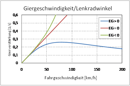
The picture shows possible courses depending on the sign of the self-steering gradient. Understeering vehicles have a maximum of the yaw gain, which is at the characteristic speed

${\displaystyle v_{ch}={\sqrt {\frac {l}{EG}}}}$

occurs. In the case EG <0, the denominator of the yaw gain can become zero. The speed at which this occurs is called the critical speed

${\displaystyle v_{krit}={\sqrt {-{\frac {l}{EG}}}}}$

designated. The yaw amplification increases beyond all limits at this point, the vehicle becomes unstable.

The maximum yaw gain in relation to the steering wheel angle has the value for understeering vehicles

${\displaystyle \left.{\frac {\dot {\psi }}{\delta _{H}}}\right|_{\mathrm {max} }={\frac {1}{i_{S}}}\cdot {\frac {1}{2\cdot {\sqrt {l\cdot EG}}}}}$.

Most cars have maximum yaw gains in the range between 0.2 1 / s and 0.4 1 / s. As a characteristic value, the maximum yaw gain describes the impression of agility of a vehicle at medium speeds (country roads). The characteristic speed for most cars is in the range between about 70 km / h and 110 km / h.

The initial slope of the yaw gain over the vehicle speed is called the static steering sensitivity . It is a measure of the maneuverability of a vehicle at low speeds. She has the value

${\displaystyle \left.{\frac {d{\frac {\dot {\psi }}{\delta _{H}}}}{dv}}\right|_{v=0}={\frac {1}{i_{S}\cdot l}}}$.

and depends only on the overall steering ratio and wheelbase. Vehicles with a short wheelbase are therefore perceived as being more agile at low speeds.

Slip angle

The slip angle can already be derived from the kinematic relationships. The following applies:

${\displaystyle {\begin{aligned}\beta &=-{\frac {l_{h}}{R}}+\alpha _{h}\\&=-{\frac {l_{h}}{R}}+\underbrace {\frac {m_{h}}{c_{h}}} _{SG}\cdot a_{y}.\end{aligned}}}$

The term is called the slip angle gradient (SG). Small sideslip angle gradients are the prerequisite for safe, stable driving behavior. The main influencing factor is the choice of tires on the rear axle. ${\displaystyle {\tfrac {m_{h}}{c_{h}}}}$

Analogous to the yaw gain, a slip angle gain can also be calculated. After some transformations the result is:

${\displaystyle {\frac {\beta }{\delta _{H}}}={\frac {1}{i_{s}}}\cdot {\frac {-l_{h}+v^{2}\cdot SG}{l+v^{2}\cdot EG}}}$.

Too high a side slip angle gain is undesirable in terms of driving dynamics, since it contributes to unsafe driving behavior at high speeds.

dynamic behaviour

In the case of dynamic behavior, transient and decay processes and the response to certain test signals are of interest. The most important are the steering angle jump and the sinusoidal excitation. These processes are characterized by their transfer functions .

To calculate these properties, it is advisable to switch to the state space representation :

${\displaystyle \mathbf {\dot {x}} =\mathbf {A} \cdot \mathbf {x} +\mathbf {B} \cdot u}$with and . ${\displaystyle \mathbf {x} ={\begin{bmatrix}\beta \\{\dot {\psi }}\end{bmatrix}}}$ ${\displaystyle u={\frac {\delta _{H}}{i_{S}}}}$

Natural frequency and damping

Transient and decay processes are determined by the natural frequency and damping . These can be calculated with the help of the eigenvalues . The eigenvalues ​​result from the characteristic polynomial

${\displaystyle \det(\mathbf {A} -\lambda \cdot \mathbf {I} )=0}$.

Written out:

${\displaystyle \lambda ^{2}-(a_{11}+a_{22})\cdot \lambda +(a_{11}\cdot a_{22}-a_{12}\cdot a_{21})=0}$

The solution to the characteristic polynomial is

${\displaystyle \lambda _{1,2}={\frac {a_{11}+a_{22}}{2}}\pm {\sqrt {\left({\frac {a_{11}+a_{22}}{2}}\right)^{2}-(a_{11}\cdot a_{22}-a_{12}\cdot a_{21})}}}$.

The stability criterion according to Hurwitz states that all coefficients of the polynomial must be positive; only the constant term can be negative. It follows:

${\displaystyle (a_{11}\cdot a_{22}-a_{12}\cdot a_{21})>0}$.

Expressed in the vehicle parameters:

${\displaystyle {\frac {c_{v}\cdot c_{h}\cdot l}{m\cdot \theta \cdot v^{2}}}\cdot (l+v^{2}\cdot EG)>0}$.

The stability condition of the single-track model is thus:

${\displaystyle l+v^{2}\cdot EG>0}$.

This condition has already been derived for the critical speed. The stationary characteristic self-steering gradient is thus also an important measure of stability .

Conventional cars have real eigenvalues ​​at low driving speeds, and conjugate complex eigenvalues ​​at medium to high driving speeds. In the case of driving speeds relevant to driving dynamics, the conjugate complex case can be assumed. The eigenvalues ​​can then be interpreted as follows:

${\displaystyle \lambda _{1,2}=-\omega _{0}\cdot D\pm j\cdot \underbrace {\omega _{0}\cdot {\sqrt {1-D^{2}}}} _{\omega _{D}}}$.

Are there

${\displaystyle \omega _{0}}$: undamped natural angular frequency ,

${\displaystyle \omega _{D}}$: damped natural angular frequency,

${\displaystyle D}$: Lehr's degree of damping ,

${\displaystyle \omega _{0}\cdot D}$: Decay constant .

A comparison with the eigenvalues ​​gives:

${\displaystyle {\begin{aligned}\omega _{0}^{2}&=(a_{11}\cdot a_{22}-a_{12}\cdot a_{21}),\\D&=-{\frac {a_{11}+a_{22}}{2\cdot \omega _{0}}}.\end{aligned}}}$

The following vehicle data are given:

designation	Formula symbol	size	Unit of measurement
Dimensions	${\displaystyle m}$	1550	kg
Yaw moment of inertia	${\displaystyle \theta }$	2800	kg m 2
Distance center of gravity - front axle	${\displaystyle l_{v}}$	1,344	m
Distance center of gravity - rear axle	${\displaystyle l_{h}}$	1,456	m
Front axle slip stiffness	${\displaystyle c_{v}}$	75,000	N / rad
Rear axle slip rigidity	${\displaystyle c_{h}}$	150,000	N / rad
Total steering ratio	${\displaystyle i_{S}}$	16	-

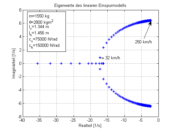
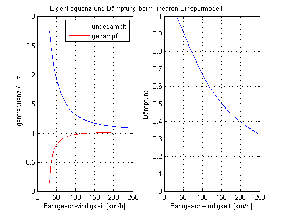
This results in the eigenvalues ​​shown in the figure depending on the driving speed. Natural frequencies and damping can be calculated from the eigenvalues. High natural frequencies and high damping are desirable, but this cannot be achieved without contradictions under the boundary conditions of the vehicle set-up.

Transfer behavior

All variables of interest (output variables) can be calculated with the aid of the state variables and the steering wheel angle input. The Laplace transformation is used for this ( complex variable). For the sake of simplicity, the same symbols are used in the image and time domains. ${\displaystyle s}$

${\displaystyle y(s)=\mathbf {C} \cdot \mathbf {x} +\mathbf {D} \cdot u}$.

An example is the transverse acceleration, the equation of which has already been shown in terms of forces and moments . The matrices and are then: ${\displaystyle \mathbf {C} }$ ${\displaystyle \mathbf {D} }$

${\displaystyle {\begin{aligned}\mathbf {C} &={\begin{bmatrix}-s\cdot v&&v\end{bmatrix}},\\\mathbf {D} &={\begin{bmatrix}0\end{bmatrix}}.\end{aligned}}}$

With:

${\displaystyle \mathbf {x} (s)={\left(s\cdot \mathbf {I} -\mathbf {A} \right)}^{-1}\cdot \mathbf {B} \cdot u=\mathbf {G} _{u}\cdot \delta _{H}}$.

Here is the vector of the transfer functions of side slip angle and yaw rate. ${\displaystyle \mathbf {G} _{u}}$

It can be shown that every transfer function has the form:

${\displaystyle {\frac {y}{\delta _{H}}}=V\cdot {\frac {Z(s)}{N(s)}}}$

can be brought.

The denominator polynomial is identical for all transfer functions and has the form:

${\displaystyle N(s)=1+{\frac {2\cdot D}{\omega _{0}}}\cdot s+{\frac {1}{\omega _{0}^{2}}}\cdot s^{2}}$.

The transfer functions can be calculated analytically using the vehicle parameters. So z. B. bring the transfer function of the yaw rate to the following form:

${\displaystyle {\dot {\psi }}(s)=V_{\dot {\psi }}\cdot {\frac {1+{}_{\dot {\psi }}\mathrm {T} _{z}\cdot s}{1+{\frac {2\cdot D}{\omega _{0}}}\cdot s+{\frac {1}{\omega _{0}^{2}}}\cdot s^{2}}}\cdot \delta _{H}}$.

The gain factor is the yaw gain already derived. The counter time constant is calculated as follows

${\displaystyle {}_{\dot {\psi }}\mathrm {T} _{z}=v\cdot {\frac {m_{h}}{c_{h}}}}$

and thus corresponds to the product of driving speed and side slip angle gradient.

Frequency response

If the complex variable is set , the frequency response is obtained from the transfer functions . The frequency response is a complex function of . The amplitude response is obtained from the amount and the phase response from the angle. The easiest way to determine the frequency responses is numerically, but they can also be specified as a function of the vehicle parameters. ${\displaystyle s=\mathrm {j} \cdot \omega }$ ${\displaystyle \omega }$

Most often, the frequency responses of yaw rate and lateral acceleration are calculated or measured while driving. When measuring in the vehicle, it must be taken into account that the acceleration is location-dependent and must therefore be converted from the measurement location to the center of gravity.

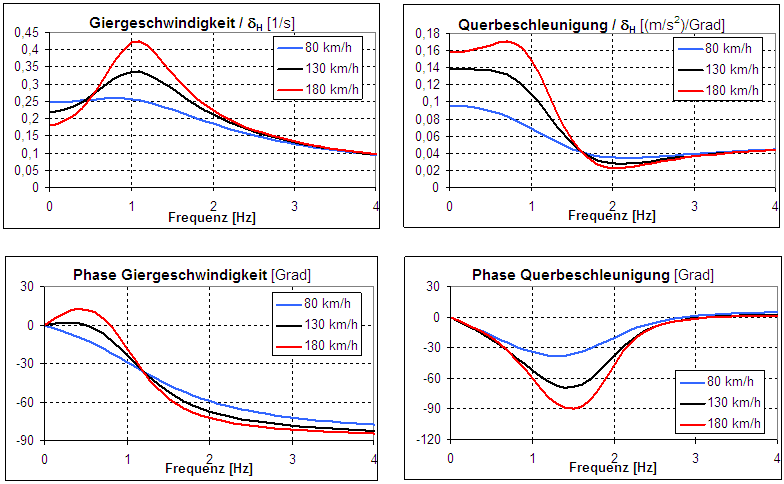
With the vehicle data from the table above, the frequency responses of yaw rate and lateral acceleration show a strong dependence on the driving speed.

The strong increase in the amplitude response of the yaw rate can be explained not only by the damping, which decreases with increasing driving speed, but also by the numerator time constant. An effective measure to improve the dynamic properties is therefore the smallest possible float angle gradient.

Mathematical derivation

Equations of motion

The equations of motion are, expressed in the state variables:

${\displaystyle {\begin{aligned}{\dot {\beta }}&=-{\frac {c_{v}+c_{h}}{m\cdot v}}\cdot \beta +{\frac {m\cdot v^{2}-(c_{h}\cdot l_{h}-c_{v}\cdot l_{v})}{m\cdot v^{2}}}\cdot {\dot {\psi }}-{\frac {c_{v}}{m\cdot v}}\cdot {\frac {\delta _{H}}{i_{S}}},\\{\ddot {\psi }}&=-{\frac {c_{h}\cdot l_{h}-c_{v}\cdot l_{v}}{\theta }}\cdot \beta -{\frac {c_{h}\cdot {l_{h}}^{2}+c_{v}\cdot {l_{v}}^{2}}{\theta \cdot v}}\cdot {\dot {\psi }}+{\frac {c_{v}\cdot l_{v}}{\theta }}\cdot {\frac {\delta _{H}}{i_{S}}}.\end{aligned}}}$

The matrices already introduced above are therefore:

${\displaystyle \mathbf {A} ={\begin{bmatrix}-{\frac {c_{v}+c_{h}}{m\cdot v}}&{\frac {m\cdot v^{2}-(c_{h}\cdot l_{h}-c_{v}\cdot l_{v})}{m\cdot v^{2}}}\\-{\frac {c_{h}\cdot l_{h}-c_{v}\cdot l_{v}}{\theta }}&-{\frac {c_{h}\cdot {l_{h}}^{2}+c_{v}\cdot {l_{v}}^{2}}{\theta \cdot v}}\end{bmatrix}}{\text{, }}\mathbf {B} ={\begin{bmatrix}-{\frac {c_{v}}{m\cdot v}}\\{\frac {c_{v}\cdot l_{v}}{\theta }}\end{bmatrix}}}$.

In state space representation:

${\displaystyle \mathbf {\dot {x}} =\mathbf {A} \cdot \mathbf {x} +\mathbf {B} \cdot u}$.

Stationary vehicle reactions

During stationary travel, the derivatives of the state variables become zero. The state variables are thus calculated

${\displaystyle \mathbf {x} =-\mathbf {A} ^{-1}\mathbf {B} \cdot u}$.

Expressed in the components of the matrices and : ${\displaystyle \mathbf {A} }$ ${\displaystyle \mathbf {B} }$

${\displaystyle {\begin{aligned}\mathbf {x} &=-{\frac {1}{\det \mathbf {A} }}{\begin{bmatrix}a_{22}\cdot b_{11}-a_{12}\cdot b_{21}\\-a_{21}\cdot b_{11}+a_{11}\cdot b_{21}\end{bmatrix}}\cdot u\\&={\begin{bmatrix}K_{\beta }\\K_{\dot {\psi }}\end{bmatrix}}\cdot u.\end{aligned}}}$

After some transformations (see also Inverse Matrix #Calculation ) the result is:

${\displaystyle {\begin{aligned}\mathbf {x} &={\begin{bmatrix}{\frac {{\frac {m_{h}}{c_{h}}}\cdot v^{2}-l_{h}}{l+v^{2}\cdot EG}}\\{\frac {v}{l+v^{2}\cdot EG}}\end{bmatrix}}\cdot u\\&={\begin{bmatrix}V_{\beta }\\V_{\dot {\psi }}\end{bmatrix}}\cdot \delta _{H}.\end{aligned}}}$

Calculation of the transfer functions

Starting from the equation

${\displaystyle \mathbf {x} (s)={\left(s\cdot \mathbf {I} -\mathbf {A} \right)}^{-1}\cdot \mathbf {B} \cdot u}$

we get, expressed in the components of the matrices and , ${\displaystyle \mathbf {A} }$ ${\displaystyle \mathbf {B} }$

${\displaystyle \mathbf {x} (s)=-{\frac {1}{\det \mathbf {A} \cdot N(s)}}{\begin{bmatrix}a_{22}\cdot b_{11}-a_{12}\cdot b_{21}-s\cdot b_{11}\\-a_{21}\cdot b_{11}+a_{11}\cdot b_{21}-s\cdot b_{21}\end{bmatrix}}\cdot u}$

With

${\displaystyle N(s)=1-{\frac {a_{11}+a_{22}}{\det \mathbf {A} }}\cdot s+{\frac {1}{\det \mathbf {A} }}\cdot s^{2}}$.

With the previously calculated reinforcements we get:

${\displaystyle \mathbf {x} (s)={\frac {1}{N(s)}}{\begin{bmatrix}K_{\beta }\cdot \left(1+{\frac {b_{11}\cdot s}{a_{12}\cdot b_{21}-a_{22}\cdot b_{11}}}\right)\\K_{\dot {\psi }}\cdot \left(1+{\frac {b_{21}\cdot s}{a_{21}\cdot b_{11}-a_{11}\cdot b_{21}}}\right)\end{bmatrix}}\cdot u.}$

Rear axle steering

The deflection on the rear axle is treated as a further independent input variable in the same way as the front axle. The input variable and the vector are expanded: ${\displaystyle u}$ ${\displaystyle \mathbf {B} }$

${\displaystyle \mathbf {u} ={\begin{bmatrix}\delta _{v}\\\delta _{h}\end{bmatrix}},\,\mathbf {B} ={\begin{bmatrix}-{\frac {c_{v}}{m\cdot v}}&-{\frac {c_{h}}{m\cdot v}}\\{\frac {c_{v}\cdot l_{v}}{\theta }}&-{\frac {c_{h}\cdot l_{h}}{\theta }}\end{bmatrix}}}$

The steering angle is the difference between the turns of the front and rear axles:

${\displaystyle \delta =\delta _{v}-\delta _{h}}$

With these extensions, formally stationary and unsteady quantities can be calculated as before. Since the driving behavior must be predictable for the driver, a fixed relationship between the steering wheel angle and the rear axle angle is required, at least when stationary ( ECE R 79 ). This is of special cases such. B. with forklifts apart from a control unit ( steer-by-wire ) calculated depending on the driving speed. If one assumes, greatly simplified, a proportional relationship between the rear axle angle and the front axle angle, which is given by the factor , the following results for the overall steering ratio : ${\displaystyle k(v)={\tfrac {\delta _{h}}{\delta _{v}}}}$

${\displaystyle i_{S}={\frac {i_{v}}{1-k(v)}}}$

In this way, important parameters such as the yaw gain, which are related to the steering wheel angle, can be generalized. Since the steering ratio is now speed-dependent, the maximum yaw gain can no longer be easily calculated.

In order to improve driving stability, an impact in the same direction (k> 0) is required. In vehicles with optional rear-axle steering, this is partially corrected by a more direct steering ratio on the front axle or superimposed steering .

literature

• Adam Zomotor: Chassis technology: driving behavior . 2nd Edition. Vogel, Würzburg 1991, ISBN 3-8023-0774-7 .
• Manfred Mitschke, Henning Wallentowitz: Dynamics of motor vehicles . 5th edition. Springer Vieweg, Wiesbaden 2014, ISBN 978-3-658-05067-2 .
• Erich Schindler: Driving dynamics . 2nd Edition. expert verlag, Renningen 2013, ISBN 978-3-8169-3188-1 .
• Dieter Schramm, Manfred Hiller, Roberto Bardini: Modeling and simulation of the dynamics of motor vehicles . Springer, Berlin / Heidelberg 2010, ISBN 978-3-540-89313-4 .

Individual evidence

1. ↑ P. Riekert, TE Schunck: On the driving mechanics of the rubber-tired motor vehicle , Ingenieur-Archiv, 11, 1940, pp. 210–224.
2. ↑ L. Diebold, W. Schindler, et al .: Single-track model for vehicle dynamics simulation and analysis , ATZ online, edition 2006-11.
3. ↑ Erich Schindler: Driving dynamics: Fundamentals of steering behavior and their application for vehicle control systems . expert verlag, 2007, ISBN 978-3-8169-2658-0 , p. 34 . ( limited preview in Google Book search)
4. ^ Karl-Ludwig Haken: Fundamentals of automotive engineering . 4th edition. Hanser, 2015, ISBN 978-3-446-44216-0 , pp. 252 . ( limited preview in Google Book search)
5. ^ Mitschke, Manfred: Dynamics of Motor Vehicles; Springer-Verlag 2004; ISBN 3-540-42011-8
6. ^ Otto Föllinger: Control engineering , 5th improved edition, Hüthig-Verlag 1985.