
HDRI generation from exposure series
In digital photography , an HDR image with a high brightness range can be generated from a series of exposures of conventional images with a low brightness range (LDR images). Since today's HDR image sensors and cameras are very expensive, this technology, in conjunction with conventional digital cameras, is the means of choice for generating HDR images at low cost.

principle
If a scene was captured several times with different exposure times , each image will contain different pixels that have been overexposed or underexposed . To generate an HDR image, it is assumed that the brightness and color of most of the pixels are correctly reproduced in at least one image in the series.
Assuming that the camera responds linearly to brightness, each individual image can be brought to the same brightness unit by dividing its pixel values by the exposure time. An HDR image can then be generated by calculating the mean value of the individual images excluding the overexposed and underexposed pixels. The conversion of the HDR image generated in this way into an LDR image for display on conventional screens is done using tone mapping .
In practice, digital cameras do not have a linear response behavior, but are characterized by a "camera curve" ( opto-electronic transfer function, also opto-electronic conversion function or OECF), which indicates how the camera reacts to different brightnesses. In addition, neither the camera nor the objects depicted are usually completely still. In addition, the camera optics scatter some of the light, which leads to undesirable lens flare effects that have to be corrected. An HDR image can also be created from negative films that have been exposed and developed for different lengths of time , whereby some of these problems do not occur here (see also Multi-Exposure ), others appear different and have to be calculated when taking the picture, for example the Schwarzschild factor and color correction .


f / 4 - 1 sec.

f / 4 - 1/4 sec.
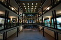
f / 4 - 1/8 sec.

f / 4 - 1/15 sec.

f / 4 - 1/30 sec.


technology
Weighting of the pixels
When combining the individual images into an HDR image, the overexposed and underexposed pixels must be ignored, but this leaves the question of how the pixels with an intermediate brightness should be weighted in relation to the pixels of the other individual images. Various methods have been proposed for this purpose.
Mann and Picard assumed that a higher sensitivity in the response behavior of the image sensor leads to a more reliable brightness value, and therefore proposed the derivation of the camera curve as a weighting function . Debevec and Malik, on the other hand, avoided the steep gradients of the camera curve at very low and high brightness values and used a function that descends to the extremes for weighting, which gives preference to pixels with a medium brightness value. Mitsunaga and Nayar used signal-theoretic arguments to show that higher values are less susceptible to noise, so they multiplied Mann and Picard's function by the pixel value. Mitsunaga and Nayar's weighting function can be multiplied by Debevec and Malik's function to avoid dubious intensity values close to the extremes.
Position alignment
Since the camera often wobbles when taking the individual images, even when using a tripod, blurring occurs when the individual images are merged unless their position is adjusted beforehand. Although various techniques have been developed in the area of machine vision in order to match several images, only a few deal specifically with the problem of HDR generation.
Motion estimation
Kang et al. solve the problem of position adjustment using a variant of the motion estimation algorithm by Lucas and Kanade (see Lucas-Kanade method ). A motion vector is determined for each pixel between two successive individual images and is then corrected. As soon as the motion vector has been determined for each pixel, successive individual images are deformed and can be merged.
The advantage of this method is that larger movements of both the camera and the objects are compensated. It is therefore suitable for recording HDR videos, whereby several differently exposed recordings are combined to form a single HDR image of the video. A disadvantage of the method is that the camera curve must be known in order to be used.
Other position adjustment methods that can correct for changes in perspective or rotations have been developed by Candocia and Kim and Polleyfeys.
Threshold bitmap
A simple and fast technique that does without the camera curve uses a so-called mean threshold bitmap. In this case, black and white images are generated from the individual images, the shifting of which relative to an arbitrarily determined reference image can easily be calculated.
To do this, each individual image is first converted into a grayscale image. A threshold value bitmap is then calculated from this , using the median of the brightness as the threshold value. For very bright or dark images, different thresholds are used to avoid excessive noise. In contrast to edge detection filters , threshold value bitmaps offer a consistent image of the recorded scene even with different exposure times.
In addition, further bitmaps are calculated in the same way from versions of the grayscale image reduced by a power of two. Based on the smallest image versions in each case, the XOR difference to the reference bitmap is calculated, whereby the bitmap can be shifted by ± 1 pixel in the X and Y axes. Image areas with a grayscale value close to the threshold value are ignored because they are often noisy in the bitmap. This is repeated for each next larger image version, the shifts taking place in addition to the position that resulted in the smallest XOR difference in the previous step. In the end, the position of the image relative to the reference image can be determined.
The threshold technology only helps against camera shake and cannot be used for individual moving objects and larger zooms or rotations of the camera.
Evaluation of the camera curve

The inverse function of the camera curve must be applied to the pixel values of the individual images before they are combined to form an HDR image in order to obtain linear brightness values. This feature is generally not published by camera manufacturers. An sRGB - tone curve is not a viable assumption since most manufacturers increase the color contrast using the sRGB curve addition, to obtain a living looking image. Also, the curve is often shifted towards the extremes to get softer highlights and less noticeable noise in dark areas. If the behavior of the camera does not change as a function of the exposure time, it is possible to determine the camera curve from a series of images with different exposure times. It is recommended to determine the function only once based on a scene with many neutral gray tones and then to use it again for all scenes.
The different values that each point of the image assumes as a function of the exposure time represent an approximation of the camera curve. Since the exposure times of the individual images are known, the curve can be reconstructed. The picture opposite shows the camera curve, which was evaluated at three different image positions with five different exposure times each. It is true that the shape of the curve can be determined in each area, but not how the individual curve sections are connected to one another. Debevec and Malik solve this problem by linear optimization , i.e. by calculating the parameters of an objective function that minimize the mean square deviation from the points. The three RGB color channels are treated independently of one another. A somewhat more elaborate procedure was published by Mitsunaga and Nayar. The objective function also takes into account variable ratios of successive exposure times. This allows the camera curve to be approximately reconstructed even in the case of inexpensive digital cameras in which the aperture number and exposure time are not precisely known.
These techniques use a series of image positions that cover the entire brightness range as well as possible. While it would be possible to use all the pixels in the image, doing so would be inefficient and create instability due to image noise. Instead, it is preferred to strategically select a number of small image regions, each with approximately the same brightness (Reinhard et al. Give 50 regions of 12 × 12 pixels each as a guideline). For this purpose, the image with the shortest exposure time is assumed. For each image it is determined how many regions of the previous image are still valid and how many must be newly selected. The required new regions are then selected at random, ensuring that they are brighter than all previous ones, do not overlap any regions that already exist and are in the brightness range that is valid for the current exposure time.
Handling of moving objects
If objects or people moved in the scene during the recording of the individual images, they appear blurred in the combined HDR image. The motion estimation technique by Lucas and Kanade tries to solve this problem by deforming image regions, but it can leave empty image regions and is powerless with complex movements. Another possibility is to select only one single image for those regions in which the image content changes; the HDR properties are then lost in these regions. This method only provides usable results if the brightness is approximately uniform in the regions concerned.
In order to automatically recognize the image regions with motion component, the weighted variance of all individual images can be calculated for each pixel . In this variance image, a “background image ” with low variance and contiguous regions with high variance are determined using flood fill . The single image to be selected for a region is that which contains the brightest areas occurring in the region with the highest possible exposure time. So that areas with low variance remain within a region, interpolation is carried out between the original HDR image and the selected individual image depending on the variance of a pixel. The result is often not perfect, as artifacts such as missing object parts can occur.
Filtering the lens scatter
Most digital cameras contain optics designed to take LDR images. Even with the use of high quality cameras, these limitations become apparent in the form of lens flare . The lens spread can be approximated by the point spread function (PSF). This function indicates the observed radially symmetrical light fall-off from a point light source in a completely dark environment. It is influenced by many parameters and can vary depending on the image. It is therefore preferred to determine the PSF from each newly captured HDR image.
To calculate the PSF on the basis of an HDR image, one takes advantage of the fact that there are a few dark pixels next to very light pixels in the image. The PSF can be approximated by determining the minimum pixel values that are located at certain distances from all light pixels. To do this, the minimum pixel value at a certain distance is divided by the value of the light pixel. It must be taken into account here that bright pixels can be close to one another and thus the circles defined by a certain radius overlap one another.
As soon as the PSF has been determined, the lens spread can be filtered out by subtracting the PSF weighted by the pixel value from its surroundings for each pixel.
HDRI generation with the scanner
An optimally exposed and developed negative can contain a contrast range of up to 12 f-stops, which cannot be completely captured in a single scan when digitizing with a film scanner due to the hardware. Multi-Exposure is a process for obtaining the largest possible dynamic range when scanning transparencies such as slides, negatives and film strips. The original is scanned several times, but with different exposures. The HDR scan is then calculated from the individual scans.
literature
- Jürgen Held: HDR photography. The comprehensive manual. 4th edition, Rheinwerk Verlag, Bonn 2015, ISBN 978-3-8362-3012-4
- Reinhard Wagner: Professional book HDR photography , pp. 107–157. Dpunkt, Heidelberg 2008, ISBN 3-89864-430-8
- Erik Reinhard u. a .: High Dynamic Range Imaging, pp. 117-159. Morgan Kaufman, San Francisco 2006, ISBN 0-12-585263-0
Web links
- Homepage of Paul Debevec (English)
- Fotocommunity.de: DRI (see "Second procedure")
Individual evidence
- ^ S. Mann, RW Picard: Being “Undigital” with Digital Cameras: Extending Dynamic Range by Combining Differently Exposed Pictures. In IS & T's 48th annual conference, pp. 422-428. Society for Imaging Science and Technology, Washington DC 1995
- ^ A b Paul Debevec, Jitendra Malik: Recovering High Dynamic Range Radiance Maps from Photographs. In SIGGRAPH 97 Conference Proceedings, pp. 369-378. ACM SIGGRAPH, New York 1997, ISBN 0-89791-896-7 ( PDF, 1.4 MB )
- ↑ a b Tomoo Mitsunga, Shree K. Nayar : Radiometric SelfCalibration. In Proceedings of the IEEE Conference on Computer Vision and Pattern Recognition, Vol. 1, pp. 374-380. IEEE, Fort Collins 1999, ISBN 0-7695-0149-4 ( PDF, 950 kB )
- ↑ Reinhard u. a .: High Dynamic Range Imaging, p. 119 f.
- ↑ Sing Bing Kang et al. a .: High Dynamic Range Video. In ACM SIGGRAPH 2003 Papers, pp. 319-325. ACM, San Diego 2003, ISBN 1-58113-709-5
- ↑ a b Bruce Lucas, Takeo Kanade: An Iterative Image Registration Technique with an Application in Stereo Vision. In Seventh International Joint Conference on Artificial Intelligence (IJCAI-81), pp. 674-679. Kaufmann, Los Altos 1981, ISBN 0-86576-059-4 ( Online ; PDF; 192 kB)
- ↑ Reinhard u. a .: High Dynamic Range Imaging, p. 122
- ↑ FM Candocia: Simultaneous Homo Graphic and Comparametric Alignment of Multiple Exposure Adjusted Pictures of the Same Scene. IEEE Transactions on Image Processing 12, 12 (Dec. 2003): 1485–1494, ISSN 1057-7149 ( PDF, 880 kB ( Memento of the original dated August 6, 2007 in the Internet Archive ) Info: The archive link was inserted automatically and not yet Checked. Please check the original and archive link according to the instructions and then remove this note. )
- ↑ SJ Kim, M. Pollefeys: Radiometric Self-Alignment of Image Sequences. In Proceedings of the IEEE Conference on Computer Vision and Pattern Recognition 2004, pp. 645-651. IEEE Computer Society, Los Alamitos 2004, ISBN 0-7695-2158-4 ( PDF, 1.7 MB )
- ^ Greg Ward: Fast, Robust Image Registration for Compositing High Dynamic Range Photographs from Hand-held Exposures. Journal of Graphics Tools 8, 2 (2003): 17–30, ISSN 1086-7651 ( PDF, 4.8 MB )
- ↑ Reinhard u. a .: High Dynamic Range Imaging, p. 136
- ↑ Reinhard u. a .: High Dynamic Range Imaging, p. 145
- ↑ Reinhard u. a .: High Dynamic Range Imaging, p. 143
- ↑ Reinhard u. a .: High Dynamic Range Imaging, pp. 147-151
- ↑ Reinhard u. a .: High Dynamic Range Imaging, pp. 155-159