Threshold procedure

The threshold value methods are a group of algorithms for segmenting digital images . Segmentation in general can be an important step in image analysis, for example to identify objects in the image. With the help of threshold value methods, it is possible to decide in simple situations which pixels represent searched objects and which belong to their surroundings. Threshold methods lead to binary images .

introduction

The motivation for using binary images is usually the availability of fast binary image algorithms, for example for blob analysis ; the saving of storage space plays a smaller role in image processing applications today.

As with all segmentation methods, with the threshold value method image points - the so-called pixels  - are assigned to different groups - the so-called segments  . The image to be segmented is in the form of numerical values ​​(one or more color values ​​per pixel). The affiliation of a pixel to a segment is decided by comparing the gray value or another one-dimensional feature with a threshold value . The gray value of a pixel is its pure brightness value; further color information is not taken into account. Since this operation is mostly used independently for each pixel, the threshold value method is a so-called pixel-oriented segmentation method.

Threshold value methods are among the oldest methods in digital image processing . The well-known Otsu process described in the section of the same name was published in 1979 by Nobuyuki Otsu . However, there are older publications on this subject. Threshold value methods can be implemented quickly due to their simplicity and segmentation results can be calculated with little effort. However, the quality of the segmentation is generally worse than with more complex methods.

classification

Image segmentation is usually the first step in image analysis in the machine vision process and takes place after image preprocessing. The typical sequence in an image processing system is as follows:

Scene → image acquisition → image preprocessing → segmentation (e.g. threshold value method ) → feature extraction → classification → statement

The scene represents one or more real, observed objects. With suitable sensors , an image of the scene is generated, usually a photograph or a video recording . In principle, however, any imaging method can serve as an image source, so that, for example, radar scans or X-ray images can also be used . If the image is not in digital form, it must first be digitized by scanning, for example , in order to be able to process it further in the computer.

Image preprocessing improves the image so that the following steps can be performed more effectively. This can mean, for example, a brightness correction, the contrast can be improved or the edges sharpened. Which preprocessing operations are favorable depends on the specific procedures in the following steps. Threshold value methods are generally susceptible to changes in brightness in the image, so brightness compensation can be advantageous.

In the segmentation step, the pixels of the image are divided into segments, for which a threshold value method is used, for example. In the subsequent feature extraction, certain properties - the so-called features - are determined for each segment . Which characteristics these are depends very much on the individual case. Examples include the area, the eccentricity of the shape or the mean color value.

With the help of the characteristics and a previously determined set of rules or a previously trained classifier , each segment can now be classified in one of several classes. By interpreting this result, a final statement can be made, for example in the text recognition "The object shown is the letter 'f' and no other".

properties

Usually, the threshold value process binarizes an initial image, i.e. exactly two segments are formed - in what is probably the most common application for this process, ideally the background and the objects sought. The assignment to the two segments (0 and 1) takes place on the basis of a comparison of the gray value g of the observed pixel with the previously defined threshold value t ( English threshold means “threshold value”). The resulting image can therefore be calculated with very little computing effort , since only one simple comparison operation has to be carried out per pixel. The corresponding calculation rule in the figure is: ${\displaystyle T_{\text{global}}}$

${\displaystyle T_{\text{global}}(g)={\begin{cases}0&{\text{falls }}g<t\\1&{\text{falls }}g\geq t\end{cases}}}$

The threshold value methods are so-called complete segmentation methods, i.e. each pixel is assigned to a segment. They are also free of overlap, so no pixel is assigned to multiple segments. In contrast to many other segmentation methods, the threshold value methods do not form contiguous segments. It is quite conceivable and often wanted that several spatially separated objects in the image, which have a similar brightness value, are combined to form a segment. In practice, incorrect segmentation of individual pixels in the middle of objects also regularly occurs, which is due, for example, to image noise in the output image . The size of the segmented objects can vary greatly depending on the choice of the threshold value.

variants

Regardless of the choice of threshold value (as described in the section of the same name below), the basic principle of the threshold value method can be applied in various ways.

In the global threshold method , a threshold value is chosen globally for the entire image. The associated calculation rule was already given in the Properties section above. The procedure is the easiest to calculate, but it is also very susceptible to changes in the brightness of the image.

Threshold value methods with a global threshold are therefore only successfully used in industrial applications for high-contrast images. Such images arise, for example, when scanning originals or when taking pictures in transmitted light.

By defining several threshold values, the global method can be varied in such a way that the segmentation provides more than two segments. For n segments, (n-1) threshold values t _{i are} required:

${\displaystyle T_{{\text{global}}_{n}}(g)={\begin{cases}0&{\text{falls }}g<t_{1}\\1&{\text{falls }}t_{1}\leq g<t_{2}\\\vdots &\vdots \\n&{\text{falls }}g\geq t_{n-1}\end{cases}}}$

With the local threshold value method , the initial image is divided into regions and the threshold value is determined separately for each region. This means that a suitable threshold value t _i can be selected in each image region R _i without this affecting the quality of the segmentation in other regions. The calculation rule for each pixel (x, y) is:

${\displaystyle T_{\text{lokal}}(x,y)={\begin{cases}0&{\text{falls }}g(x,y)<t_{i}\\1&{\text{falls }}g(x,y)\geq t_{i}\end{cases}}\quad \forall (x,y)\in {\text{Region }}R_{i}}$

Compared to the global threshold value method , the complexity increases only insignificantly; the local method can therefore also be calculated with little computing effort. The susceptibility to changes in brightness decreases, but there may be an offset at the borders of the regions. Depending on the number of regions, the effort can be too high for one person to choose the appropriate threshold value for each region. An automatic procedure for selecting the threshold value is therefore advisable.

The dynamic threshold value method can be seen as a further development of the local method , which considers a neighborhood N for each pixel and calculates a suitable threshold value t (N) on the basis of this neighborhood . An automatic procedure for selecting the threshold value is absolutely necessary here. The corresponding calculation rule for each pixel (x, y) is:

${\displaystyle T_{\text{dynamisch}}(x,y)={\begin{cases}0&{\text{falls }}g(x,y)<t(N(x,y))\\1&{\text{falls }}g(x,y)\geq t(N(x,y))\end{cases}}}$

The dynamic variant is quite stable against local changes in brightness. The computational effort increases considerably here, however, since a new threshold value is calculated for each pixel.

example

• Noise image
• 

  Initial image ...

• 

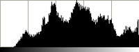
  ... and the associated histogram (logarithmic scale).

The sample image is a noisy grayscale image with fuzzy edges, as seen on the left. Blurred edges here means that the edges are not clear, but rather go through a transition from the white background to the black object and the pixels in the edge area take on different shades of gray.

The associated histogram (on the right) helps you choose the threshold value that matches the image . In a histogram, the frequency of each individual gray value is indicated by a correspondingly high line. A bar with the various gray values ​​is therefore displayed as a legend on the horizontal coordinate axis, and the height of the line above that indicates the relative frequency of occurrence of the respective gray value.

Two maxima can be clearly seen in the histogram : the dark object (left maximum) and the light background (right maximum). Every gray value between the two maxima also appears in the image, which is caused by the noise in the image and the soft object edges, where the pixels gradually take on the various gray levels from white to black.

The initial image was segmented using the global threshold value method; to demonstrate the method, the result image was calculated for four different threshold values. In the resulting binary images, each with two segment groups, each pixel was colored black (0) or white (1) according to its assignment to the object or to the background. More precisely: All pixels with gray values ​​smaller than the threshold value were colored black, all pixels with gray values ​​greater than or equal to the threshold value were colored accordingly white.

• Segmentation with a different threshold
• 

  Threshold 30

• 

  Threshold 52

• 

  Threshold 204

• 

  Threshold 230

When it is segmented with the threshold value 30, several pixels belonging to the object are colored white, that is, segmented to the background. The threshold was therefore chosen too low.

With the two threshold values ​​52 and 204, the results are quite decent. This also applies to all threshold values ​​between these two values. The difference can be seen in the fact that the object becomes slightly larger as the threshold value increases. The choice of the threshold value therefore not only influences the quality of the segmentation itself, but also the sizes of the segmented areas. The reason for the growth of the area are the pixels in the edge area, which gradually cover the gray values ​​from white to black.

The threshold 230 also segments some background pixels as belonging to the object. This is an indication that it was chosen too big.

Choice of threshold

The key point in all threshold value methods is the choice of a suitable threshold value. This can be sensibly selected by a human processor. However, since the local and dynamic threshold value method requires a larger number of threshold values, it is advisable to use an automatic method for determining the threshold values. Of course, the threshold value can also be determined automatically with the global threshold value method. There are a large number of specific methods for choosing a suitable threshold value.

The histogram is the most important aid for both manual and automatic definition of a threshold value. Local maxima indicate the gray values ​​or gray value ranges that are assumed in the image from the background or from larger objects. In the ideal case, the histogram is bimodal , that is, two clearly separated maxima can be recognized. A simple, but also error-prone approach is to choose the mean value between the two maxima as the threshold value. Another, simple approach is to define the gray value of the minimum between the maxima as the threshold value. This would probably achieve a somewhat better separation.

If you process images from the same source again and again, you can often apply a threshold value chosen once to all of these images.

One of the more sophisticated methods for the automatic determination of threshold values ​​is the Otsu method, which has established itself as a standard and will be presented below.

Procedure of Otsu

The Otsu method according to Nobuyuki Otsu from 1979 uses statistical tools to solve the problem of the best possible threshold value. In particular, use is made of the variance , which is a measure of the spread of values ​​- in this case it is about the spread of the gray values.

Otsu's method determines a threshold value at which the scatter within the classes determined by it is as small as possible, but at the same time as large as possible between the classes. For this purpose, the quotient between the two variances is formed and a threshold value is sought at which it is as large (maximum) as possible.

Mathematical representation

The starting point is two classes of points ( and ), which are separated from one another based on the threshold value sought . is the variable you are looking for, the two classes are the desired result. In the following, using the Otsu method, a measure is determined according to which the threshold value (and thus the classes) can be optimized. ${\displaystyle K_{0}(t)}$ ${\displaystyle K_{1}(t)}$ ${\displaystyle t}$ ${\displaystyle t}$

Let the probability of occurrence of the gray value be 0 <g <G (G is the maximum gray value). Then the probability of the appearance of pixels of the two classes results with: ${\displaystyle p(g)}$

${\displaystyle K_{0}}$: and : ${\displaystyle P_{0}(t)=\sum _{g=0}^{t}p(g)}$ ${\displaystyle K_{1}}$ ${\displaystyle P_{1}(t)=\sum _{g=t+1}^{G}p(g)=1-P_{0}(t)}$

Assuming two classes (i.e. a threshold value), the sum of these two probabilities is of course 1.

If the arithmetic mean of the gray values ​​is within the entire image, and and the mean values ​​within the individual classes, then the variances within the two classes result as: ${\displaystyle {\overline {g}}}$ ${\displaystyle {\overline {g_{0}}}}$ ${\displaystyle {\overline {g_{1}}}}$

${\displaystyle \sigma _{0}^{2}(t)=\sum _{g=0}^{t}(g-{\overline {g_{0}}})^{2}p(g)}$ and ${\displaystyle \sigma _{1}^{2}(t)=\sum _{g=t+1}^{G}(g-{\overline {g_{1}}})^{2}p(g)}$

The goal is now to keep the variance of the gray values ​​in the individual classes as low as possible, while the variance between the classes should be as large as possible. This results in the following quotient:

${\displaystyle Q(t)={\frac {\sigma _{zw}^{2}(t)}{\sigma _{in}^{2}(t)}}}$

The variance between the classes is:

${\displaystyle \sigma _{zw}^{2}(t)=P_{0}(t)\cdot ({\overline {g_{0}}}-{\overline {g}})^{2}+P_{1}(t)\cdot ({\overline {g_{1}}}-{\overline {g}})^{2}}$

The variance within the classes results from the sum of the two individual variances:

${\displaystyle \sigma _{in}^{2}(t)=P_{0}(t)\cdot \sigma _{0}^{2}(t)+P_{1}(t)\cdot \sigma _{1}^{2}(t)}$

The threshold value is now chosen so that the quotient is maximum. so is the amount you are looking for. If a threshold value is determined by maximizing the quotient, it divides the point sets into optimal classes according to the variance. ${\displaystyle t}$ ${\displaystyle Q(t)}$ ${\displaystyle Q(t)}$

Problems

• Brightness problems
• 

  The picture with a brightness gradient, ...

• 

  ... the associated histogram (linear scaling) ...

• 

  ... and the result of the segmentation with the threshold value 127.

The global threshold method is very sensitive to changes in brightness across the image. The three images demonstrate this problem: The original image (left) was given a brightness gradient. The histogram (middle picture) is no longer bimodal, as in the example above, no two clearly separated maxima can be made out, but there are considerably more, rather small local maxima. The result image (right) of the segmentation with the threshold value 127 is inconsistent: at the top left, entire background areas are segmented as an object, while the object at the bottom right is recognized as the background. The segmentation is roughly correct only in the middle of the image.

The application of the local or even the dynamic threshold value method could improve the segmentation result here. However, the latter in particular is much more computationally intensive. In addition, it must be ensured that all objects to be segmented occur in each region, otherwise the automatically selected threshold values ​​could be calculated incorrectly. For example, if there are three objects (and the background) in the image, three thresholds are chosen to separate the four classes. If only two of the three objects appear in a region, then the third threshold value cannot be correctly determined there. So the result of the segmentation from this region will not match well with the results from the other regions. An alternative solution would be to compensate for the brightness in a preprocessing step, for example with a shading correction or by offsetting a reference image .

In addition to brightness gradients, other image errors that can lead to segmentation problems can be eliminated or reduced by suitable image preprocessing. The noise removal from images or the sharpening of edges are often used. Post-processing can also help eliminate segmentation problems. In this way, incorrectly segmented pixels can be corrected by humans or by suitable filtering.

In contrast to many other segmentation methods, the threshold value method does not automatically result in contiguous segments; if there is a lot of noise, individual pixels are almost always segmented out.

The threshold value methods always use only one-dimensional image information (usually an intensity value or gray value). Additional information, for example different color channels, is not evaluated.

Some of these problems can be avoided by using other, sometimes more complex, methods of segmentation .

Applications

The threshold value methods are very well suited for fast binarization (separation of objects and background) of evenly illuminated images, for example scans . This means, for example, a good suitability for the first step of a text recognition .

It is included as an editing function in many image editing programs , such as GIMP , ImageJ and IrfanView .

Threshold value methods are also standard methods in digital image processing and are included in this area in every program library .

literature

• Thomas Lehmann, Walter Oberschelp, Erich Pelikan, Rudolf Repges: Image processing for medicine . Springer, Berlin / Heidelberg 1997, ISBN 3-540-61458-3 .
• Bernd Jähne : Digital image processing . 5th edition. Springer, Berlin 2002, ISBN 3-540-41260-3 .
• Rafael C. Gonzalez, Richard E. Woods: Digital Image Processing . Addison-Wesley, Reading MA 1992, ISBN 0-201-50803-6 (English).
• Nobuyuki Otsu: A threshold selection method from gray level histograms . In: IEEE Transactions on Systems, Man, and Cybernetics . New York, 9.1979, pp. 62-66. ISSN  1083-4419

Web links

• Seminar presentation on segmentation (PDF; 900 kB)

Individual evidence

1. ↑ Survey over image thresholding techniques (English; PDF; 3.0 MB)

This article was added to the list of excellent articles on November 10, 2006 in this version .