Karnaugh-Veitch diagram

Fig. 1-1: Karnaugh-Veitch diagram: ¬AB¬C¬D ∨ A¬B¬C¬D ∨ A¬B¬CD ∨ A¬BC¬D ∨ A¬BCD ∨ AB¬C¬D ∨ ABC¬ D v ABCD = AC ∨ B¬C¬D ∨ A¬B

Fig. 1-2: Karnaugh-Veitch diagram: ABCD ∨ AB¬CD ∨ ¬AB¬CD ∨ A¬BC¬D ∨ ¬A¬BC¬D ∨ ¬A¬B¬CD = ABD ∨ ¬A¬CD ∨ ¬ BC¬D

The Karnaugh-Veitch diagram (or the Karnaugh-Veitch symmetry diagram , the Karnaugh table or the Karnaugh plan ), KV diagram for short , KVS diagram or K diagram ( English Karnaugh map ), provides a clear overview Representation and simplification of Boolean functions in a minimal logical expression. It was designed in 1952 by Edward W. Veitch [ viːtʃ ] and further developed in 1953 by Maurice Karnaugh [ ˈkɑːɹnɔː ] to its present form.

properties

Any disjunctive normal form (DNF) can be converted into a minimal disjunctive logical expression using a KV diagram . The advantage over other methods is that the term generated is (mostly) minimal. If the term is not yet minimal, a further simplification is possible by applying the distributive law (bracketing). The conversion begins with the creation of a truth table , from which the DNF is derived, which in turn is converted directly into a KV diagram.

Since the minterms belonging to the neighboring fields differ in only one variable A through negation, this is eliminated (after factoring out with the distributive law and applying ) from the term that describes the neighboring fields to be summarized. The group reduction is based on this rule. ${\ displaystyle A \ vee \ neg A = 1}$

The inverse function can be found by swapping “1” and “0” in the KV diagram. ${\ displaystyle {\ bar {F}}}$

A KV diagram is also useful for identifying and eliminating hazards .

Filling out the KV diagram

A KV diagram for n input variables has 2 ⁿ fields (see example). The KV diagram is labeled with the variables on the edges. Each variable occurs in negated and non-negated form. The assignment of the variables to the individual fields can be done in any way, however, it should be noted that horizontally and vertically adjacent fields may only differ in exactly one variable ( Gray code ). With the help of the truth table of the function to be optimized, a 1 is entered in the individual fields if there is a minterm of the function , otherwise a 0. A minterm of the function is then given if applies ${\ displaystyle m}$

{\ displaystyle m ({\ underline {X}}) = 1 \ Rightarrow F ({\ underline {X}}) = 1}

,

where is the vector of the input variable. In a disjunctive normal form, this applies to every conjunction term that yields 1, since then the total disjunction and consequently also the function yields 1. ${\ displaystyle {\ underline {X}}}$

KV diagrams are suitable for simplifying functions with a maximum of approx. 4–6 input variables; up to 4 variables they are clear.

simplification

If fewer fields in the KV diagram are assigned 1 than 0, then the Minterm method is selected, otherwise the Maxterm method.

Minterm method

Fig. 2-1: Neighboring fields of the "ones" field - red fields

Fig. 2-2: Neighboring fields of the "ones" field - red fields

Fig. 2-3: Neighboring fields of the "ones" field - red fields

An attempt is made to combine as many horizontally and vertically adjacent fields as possible that contain a 1 (minterme) to form rectangular, connected blocks ( packets ). All powers of 2 are allowed as block sizes (1, 2, 4, 8, 16, 32, ...). All 1-fields are to be recorded with blocks.
A block can possibly be continued over the right or bottom edge of the diagram. This can be explained as follows: KV diagrams for three variables must basically be understood as cylinders . The fields on the far left and on the far right or above and below are therefore adjacent. KV diagrams for four variables must basically be understood as torus (“donut shape”); the four corners of the square KV diagram are adjacent. Even more complex neighborhood relationships hold for 5 or more variables. Since multidimensional structures are difficult to manipulate with drawing, one chooses the representation in the plane, but then has to keep the neighborhood relationships in mind.
Select enough blocks from the identified blocks so that all 1-fields are covered. For many switching functions, these are all combined blocks, but it is not uncommon for alternatives to exist. Then there is a free choice for blocks of the same size, otherwise the larger blocks are to be selected because they lead to the smaller (since more strongly summarized) terms.
The formed and selected blocks / packages are now converted into conjunction terms. Variables within a block that appear in negated and non-negated form are omitted.
These AND links are combined by OR links and result in a disjunctive minimal form .

Maxterm method

The Maxterm method differs from the Minterm method only in the following points:

Instead of ones, zeros are combined to form small packets.
A packet forms a disjunction term (OR operations instead of a conjunction term).
The disjunction terms are linked conjunctively (with AND).
The variables are also negated individually.

All around method

It is also possible to read off a so-called normal total form from a KV diagram. Since only minterms without negation occur in the normal round sum form, only blocks may be formed that contain no negation. By overlapping the blocks more than once, it must be achieved that all zeros are covered even often and all ones are covered odd times. Here the rule or is used. Each block provides a minterm, which are linked using XOR . The all-round normal form is unambiguous except for the order of the minterms. ${\ displaystyle T \ oplus T = 0}$ ${\ displaystyle T \ oplus T \ oplus T = T}$

Don't care states

Figure 4: Example of don't care states

There are often Boolean functions with truth tables in which a value of the output variable does not have to be defined for every combination of the input variables. Such initial states are called don't-care terms and are labeled with , because they can have the value 1 as well as 0. These fields may be viewed as 1 or 0 in order to complete blocks of ones or zeros in the Minterm or Maxterm method. A good example of this is decoding a binary coded decimal number (BCD). Only the numbers 0 to 9 play a role here, the so-called pseudotetrads can deliver any result, so they are don't care terms. ${\ displaystyle X}$ ${\ displaystyle X}$

KV diagram with several outputs

If a digital circuit has several outputs, i.e. the truth table has several columns of results, then a separate KV diagram must be created for each output.

For example, a 1-out-of-n decoder has the truth table on the right and the 4 KV diagrams on the right for its 4 outputs.

Fig. 5-1: Truth table and KV diagram for 1-out-of-n decoders

input				output
Number 1		Number 2		${\ displaystyle A <B}$	${\ displaystyle A = B}$	${\ displaystyle A> B}$
${\ displaystyle A_ {1}}$	${\ displaystyle A_ {0}}$	${\ displaystyle B_ {1}}$	${\ displaystyle B_ {0}}$	${\ displaystyle X}$	${\ displaystyle Y}$	${\ displaystyle Z}$
0	0	0	0	0	1	0
0	0	0	1	1	0	0
0	0	1	0	1	0	0
0	0	1	1	1	0	0
0	1	0	0	0	0	1
0	1	0	1	0	1	0
0	1	1	0	1	0	0
0	1	1	1	1	0	0
1	0	0	0	0	0	1
1	0	0	1	0	0	1
1	0	1	0	0	1	0
1	0	1	1	1	0	0
1	1	0	0	0	0	1
1	1	0	1	0	0	1
1	1	1	0	0	0	1
1	1	1	1	0	1	0

Another example of multiple outputs is a 2 + 2-bit comparator . It has four input variables and three output variables. The number A consists of 2 bits ( and ) and the number B consists of 2 bits ( and ). Depending on whether " ", " " or " " the three outputs output 1 or 0. ${\ displaystyle A_ {1}}$ ${\ displaystyle A_ {0}}$ ${\ displaystyle B_ {1}}$ ${\ displaystyle B_ {0}}$ ${\ displaystyle A <B}$ ${\ displaystyle A = B}$ ${\ displaystyle A> B}$ ${\ displaystyle (X, Y, Z)}$

The associated truth table is on the right. Figures 5-2 to 5-4 show the 3 KV diagrams for the 3 outputs.

Fig. 5-2: Output X

Fig. 5-3: Output Y

Fig. 5-4: Output Z

Normal forms

A.	B.	C.	D.	X
0	0	0	0	0
0	0	0	1	0
0	0	1	0	0
0	0	1	1	0
0	1	0	0	1
0	1	0	1	1
0	1	1	0	0
0	1	1	1	1
1	0	0	0	0
1	0	0	1	0
1	0	1	0	0
1	0	1	1	0
1	1	0	0	1
1	1	0	1	1
1	1	1	0	0
1	1	1	1	1

Usually groups are formed for the ones (Fig. 6-2). The ones are derived from the disjunctive normal form (DNF). But there is also the possibility of forming groups from the zeros (in Fig. 6-1 and the following, the zeros are not shown separately, but are still there). The zeros stand for the conjunctive normal form (CNF).

The DNF is: ¬AB¬C¬D ∨ ¬AB¬CD ∨ ¬ABCD ∨ AB¬C¬D ∨ AB¬CD ∨ ABCD.

The CNF is: (A∨B∨C∨D) ∧ (A∨B∨C∨¬D) ∧ (A∨B∨¬C∨D) ∧ (A∨B∨¬C∨¬D) ∧ (A ∨¬B∨¬C∨D) ∧ (¬A∨B∨C∨D) ∧ (¬A∨B∨C∨¬D) ∧ (¬A∨B∨¬C∨D) ∧ (¬A∨B ∨¬C∨¬D) ∧ (¬A∨¬B∨¬C∨D).

The DNF is read from the table by writing down each line with the output value “one”. The input variables for which a zero stands are taken in negated form. All terms for the lines (in this example 6 lines) are connected by "∨".

For the KNF, all lines with the output value "zero" are written out, whereby input variables for which a "one" stands are taken in negated form. All terms for the lines (in this example 10 lines) are connected by "∧", the literals themselves are connected by "∨".

Picture 6-1

Fig. 6-2: Polynomial BD ∨ B¬C¬D
( minimal polynomial : B (D ∨ ¬C¬D) )

Fig. 6-3: (¬C ∨ D) ∧ B

Error in Fig. 6-2: The minimal polynomial is: B (D ∨ ¬C) , because the red two-box can be expanded upwards to a four-box, whereby more literals are omitted and the final minimum polynomial of length 4 ( BD ∨ B¬C ) arises. It is important to note here that although two relevant indices are used multiple times, this is both permitted and necessary in order to form the minimal polynomial.

Laws of reduction

By combining them into a group of size 2 ⁿ , the logical expression is reduced by n variables. This is independent of the position or shape of the group or whether it extends over the edges. This is also independent of whether it is a 2 × 2, 2 × 4, 4 × 4 or 4x4x4 KV diagram.

A group of eight (2 ³ ) is reduced by 3 variables (n = 3) - Figure 9-1.
A group of four (2 ² ) is reduced by 2 variables (n = 2) - Fig. 9-2 and 9-3.
A group of two (2 ¹ ) is reduced by 1 variable (n = 1) - Figure 9-4 and 9-5.
A unit group (2 ⁰ ) is reduced by zero variables (n = 0) - Figure 9-6.

Fig. 9-1: Result: D

Fig. 9-2: Result: CD

Fig. 9-3: Result: B¬D

Fig. 9-4: Result: AB¬C

Fig. 9-5: Result: ¬B¬C¬D

Fig. 9-6: Result: ¬ABCD

Rules for group formation

Adjacent fields in which a one is entered are combined into groups.
A group cannot contain any fields with zeros. (Often the zeros are not recorded and the fields are left blank. In this case, a group must not contain any empty fields.)
All ones must be grouped together.
Adjacent fields with ones are combined into a group. (Fields that touch at the corners, diagonally, do not count as adjacent.)
The groups must be as large as possible.
As few groups as possible have to be formed.
The groups may only have sizes that correspond to powers of two (1, 2, 4, 8, 16, 32, 64 ...).
The groups must be rectangular blocks.
The groups are allowed to overlap.
The groups are allowed to go over the edges.
Two groups cannot contain exactly the same ones.
No group may be completely enclosed by another group.

Summary: One looks for a complete covering of the ones with the largest possible rectangular blocks.

KV tables for 2 and 4 variables

Image 1

picture 2

Anyone who frequently works with the KV diagram would like a method to be able to fill out a KV diagram quickly.

This is achieved with the arrangement shown above for the four input variables A , B , C and D by the following arrangement:

picture 3

Picture 4

Examples of summaries

Figure 3: Clarifies the logical values of the 16 fields; If you transfer the DNF line by line from a truth table to the KV diagram, the entry is made in the order of the red numbers
Fig. 4: The red numbers make it easier to assign the truth table to the individual fields line by line; the order depends on the specific labeling of the KV diagram; The numbering makes work easier when using KV diagrams extensively

Each field is assigned its value. With 4 signals there are 16 entries:

0000 = 0, 0001 = 1, 0010 = 2, ..., 1110 = 14, 1111 = 15

In this way, the KV diagram can be filled out very quickly. In addition to the arrangements shown above, variations in the arrangement of the input variables A , B , C and D are also possible. This results in other classifications of the values in the matrix.

Quantity diagram

The Karnaugh map is a modified, abstract form of the amount of the diagram (Venn diagram).

Figures 1 to 4 show a Venn diagram and the equivalent KV diagram.

2 variables
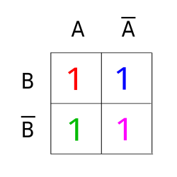
Figure 1: KV diagram
Fig. 2: Venn diagram

4 variables
Figure 3: KV diagram
Fig. 4: Venn diagram

Figures 5 to 8 once again show the individual subsets that make up the Venn diagram in Figure 4.

4 variables
Figure 5: Subset in the Venn diagram
Figure 6: Subset in the Venn diagram
Figure 7: Subset in the Venn diagram
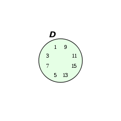
Figure 8: Subset in the Venn diagram

Visualization through hyper-unity cube

Fig. 3-1: Hypercube

Boolean functions with n variables can be illustrated graphically using unit cubes of dimension n. Cubes of any dimension are also known as hypercubes . Since Karnaugh diagrams are themselves a special form of representation for Boolean functions, it is not surprising that a clear connection can be made between hyper-unit cubes and Karnaugh diagrams. Namely, Karnaugh diagrams for n variables correspond to the hyper-unit cubes of dimension n in a reversible manner . The corner coordinates of the hyper-cube correspond to the dual numbers of the fields in the Karnaugh diagram.

Figure 3-2 shows the unit cube for 3 variables. This corresponds to a 2 × 4 KV diagram. The KV diagram in Figure 3-3 is marked accordingly in Figure 3-4 (green level). The nodes (corner points or circles) on the hyper-unit cube each correspond to a field in the KV diagram. The transitions (neighborhood of the fields) are symbolized by the edges of the cube. A Gray code is created when walking on the edge . Exactly 1 bit changes on each edge. An essential property is that the Gray codes for two neighboring numbers only differ by 1 digit, i.e. 1 bit for binary codes ( Hamming distance ).

The KV diagram has as many neighborhoods as the cube has edges. Figure 3-5 shows a planar representation of the hyper-unit cube. Without changing its internal structure of the transitions, the cube can be "turned inside out" in any direction, as shown in the animation in Figure 3-9. This explains why there are KV diagrams with different arrangements of the variables (edge labeling). They were practically "turned inside out" like a cube.

Picture 3-2

Picture 3-3

Picture 3-4

Picture 3-5

For the KV diagram with 2 variables (2 × 2 field) there is a simpler hyper-unit cube (Fig. 3-6). With 1 variable, the “cube” is trivial (Fig. 3-7). However, the number of edges increases exponentially as the variables increase. With 4 variables (Fig. 3-8) there are already 32 edges.

Picture 3-6

Picture 3-7

Picture 3-8

Picture 3-9

Extension of the symmetry diagram for more than 4 input variables

Derivation of the KV diagram by mirroring

A disadvantage of the original variant of the KV diagram is that it is not suitable for more than 4 input variables. The generalized form of the symmetry diagram can be used to work with any number of input variables.

With this method, the creation of a KV diagram with n input variables is explained by the fact that a KV diagram with n-1 input variables is mirrored and thus doubled. Hence the name "symmetry diagram". The newly created half of the KV diagram then corresponds to the newly added input variable in non-negated form, while the already existing half corresponds to the input variable in negated form.

By mirroring a symmetry diagram with n input variables, one with n + 1 input variables can be generated in this way, so that the number of input variables is not limited even in the two-dimensional area.

The formation of groups from connected, rectangular blocks in the conventional KV diagram is also explained using the mirroring:

Every conceivable group of fields in a KV diagram with n input variables, which represents a Minterm or Maxterm, can be generated by mirroring and / or maintaining a group in the KV diagram with n-1 input variables. For example, the Minterm ¬AB (marked in red in the drawing) is generated by

the original group is not included in the first mirroring (but retained),
in the second mirroring the group is also mirrored and the existing fields are not retained and
in the third mirroring, the group is also mirrored and the existing fields are retained at the same time.

Valid and invalid groups in a symmetry diagram with 6 input variables

The condition that several fields can form a group is therefore not that they are contiguous rectangular blocks, but rather whether it is possible to create a corresponding group by mirroring and retaining. In the case of KV diagrams with up to 4 input variables, this condition leads to the same groups as the rule that the groups must be connected rectangles. However, this is no longer the case with 5 input variables or more, as can be seen from the following example with 6 input variables.

The block marked in blue does not represent a valid block (which represents a minterm), although all the rules for a block formation in a conventional KV diagram would be met. The group of fields marked in red corresponds to the Minterm ¬AB¬D; it is therefore a valid group. It is clearly not a contiguous block.

However, the application of the method for more than 4 input variables is more difficult than the application with a maximum of 4 input variables, since the user does not notice unrelated groups of ones as easily as connected rectangles made of ones.

literature

Maurice Karnaugh: The Map Method for Synthesis of Combinational Logic Circuits. Transactions of the AIEE, vol. 72, no. 9 (1953), pp. 593-599.
Edward W. Veitch: A chart method for simplifying truth functions. Proc. Assoc. for Computing Machinery, Pittsburgh May 1952, pp. 127-133.
Klaus Beuth: Digital technology. Vogel Buchverlag, 2001, ISBN 3-8023-1755-6 (Chapter 5).
Günter Wellenreuther, Dieter Zastrow: Control technology with PLC: From the control task to the control program. Vieweg + Teubner Verlag, 1998, ISBN 3-528-44580-7 (Chapter 4.5.2).
Ulrich Tietze, Christoph Schenk: Semiconductor circuit technology . 12th edition. Springer, 2002, ISBN 3-540-42849-6 .
Manfred Seifart, Helmut Beikirch: Digital circuits . 5th edition. Technology, 1998, ISBN 3-341-01198-6 .

Web links

Wikibooks: Karnaugh-Veitch Diagram: Examples (Part 1) - Learning and teaching materials

Commons : Karnaugh maps - collection of images, videos and audio files

Individual evidence

↑ Hans Martin Lipp, Jürgen Becker: Fundamentals of digital technology. Oldenbourg-Verlag, Munich 2011, ISBN 978-3-486-59747-9 .

[1] Hans Martin Lipp, Jürgen Becker: Fundamentals of digital technology. Oldenbourg-Verlag, Munich 2011, ISBN 978-3-486-59747-9 .