Depth first search

Animation of depth first search in a tree

Depth-first search ( English depth-first search , DFS ) is in the computer science a method for searching of nodes in a graph . It is one of the uninformed search algorithms . In contrast to the breadth- first one is in the depth-first search path completely trodden in depth before branching paths be taken. All accessible nodes of the graph should be visited. For graphs with potentially few, long paths, the limited depth search is recommended , in which each path is only followed up to a certain depth.

An improvement in depth-first search is iterative depth-first search .

General

The depth-first search is an uninformed search algorithm which, by expanding the first occurring successor node in the graph, gradually searches further deeper from the start node. The order in which the successors of a node are determined depends on the representation of the successors . In the case of representation using an adjacency list using a linked list , for example, the nodes are traversed in the order of their entry in this list . In the picture above, it is implicitly assumed that the successors are selected from left to right.

The procedure for undirected graphs is as follows: First, a start node is selected. From this node , the first edge is now examined and tested whether the opposite node has already been discovered or is the element sought. If this is not yet the case, the depth-first search is called recursively for this node, which means that the first successor of this node is expanded again. This type of search is continued until the element searched for has either been found or the search has arrived at a sink in the graph and thus cannot examine any further successor nodes. At this point the algorithm now returns to the node that was expanded last and examines the next successor of the node. If there are no more successors here, the algorithm goes back to the respective predecessor step by step and tries again there. The animation shows an example of the application of depth first search to a tree . ${\ displaystyle \ left.u \ right.}$ ${\ displaystyle \ left (u, v \ right)}$ ${\ displaystyle \ left.v \ right.}$ ${\ displaystyle \ left.u \ right.}$

The edges of the graph used by the algorithm to traverse the graph are called tree edges . Those edges that are not used and lead from one node to another node in the same subtree that will be visited later in the depth-first search are called forward edges . Those edges that are not used and lead from one node to another node in the same subtree that was previously visited in the depth-first search are called backward edges . Those edges that run “across” from one subtree to another are called transverse edges . Within the depth-search tree , the path between two nodes connected by a transverse edge would first require an ascent and then a descent in the tree . Forward edges, backward edges, transverse edges and tree edges result in the total number of edges in the graph.

Algorithms

Determine the node where you want the search to begin
Expand the node and save the smallest / largest (optionally) not yet developed successor in a stack in the order
Call DFS recursively for each of the nodes in the stack
- If the element you were looking for was found, cancel the search and return a result
- If there are no more undeveloped successors , delete the top node from the stack and call DFS for the now top node in the stack

DFS(node, goal) {
  if (node == goal) {
    return node;
  } else {
    stack:= expand (node)
    while (stack is not empty) {
      node':= pop(stack);
      DFS(node', goal);
    }
  }
}

Creation of the depth search forest

The following recursive algorithm creates the depth-first search forest of a graph G by setting discovery and finishing times and coloring the nodes . Based on Cormen et al. first all nodes are colored white. Then, by definition, the depth-first search starts at the alphabetically smallest node and colors it gray. Then, as described above, its white neighbor is recursively considered and colored gray. If there is no longer a white neighbor, backtracking occurs , during which all nodes that have migrated through are colored black.

DFS(G)
1   for each v of G {        // Alle Knoten weiß färben, Vorgänger auf nil setzen
2      col[v] = 'w';
3      pi[v] = nil;
4   }
5   time = 0;
6   for each u of G          // Für alle weißen Knoten: DFS-visit aufrufen
7      if col[u] == 'w'
8         DFS-visit(u);

DFS-visit(u)
1   col[u] = 'g';            // Aktuellen Knoten grau färben
2   time++;                  // Zeitzähler erhöhen
3   d[u] = time;             // Entdeckzeit des aktuellen Knotens setzen
4   for each v of Adj[u] {   // Für alle weißen Nachbarn des aktuellen Knotens
5       if col[v] == 'w' {
6          pi[v] = u;         // Vorgänger auf aktuellen Knoten setzen
7          DFS-visit(v);      // DFS-visit aufrufen
8       }
9       if col[v] == 'g'{
10         // Zyklus entdeckt
11      }
12    }
13   col[u] = 's';           // Aktuellen Knoten schwarz färben
14   time++;
15   f[u] = time;            // Finishing-Time des aktuellen Knotens setzen

The time stamp (see lines 2, 14, 15) can still be used for a topological sorting . After a node has been colored black, it is added to a list , descending according to the values f [u] for the time stamp, and a topological order is obtained. If a cycle (see line 9) is discovered, this is no longer possible.

properties

In the following, the memory requirements and runtime of the algorithm are specified in Landau notation . We also assume a directed graph .

Storage space

The memory requirement of the algorithm is specified without the memory space for the graph as it is transferred, because this can be in different forms with different memory requirements, e.g. B. as a linked list , as an adjacency matrix or as an incidence matrix .

For the DFS (G) procedure described above, all nodes are first colored white and the references for their predecessors are removed. So this information requires constant for each node space , so . Overall, there is a linear memory requirement of , depending on the number of nodes (English vertices ). The memory requirement of the variable time is negligible with constant compared to . The DFS-visit (u) procedure is then called for each node u . Since these are only control structures, they do not contribute to memory requirements. ${\ displaystyle {\ mathcal {O}} (1)}$ ${\ displaystyle {\ mathcal {O}} (\ vert V \ vert)}$ ${\ displaystyle \ vert V \ vert}$ ${\ displaystyle {\ mathcal {O}} (1)}$ ${\ displaystyle {\ mathcal {O}} (\ vert V \ vert)}$

The DFS-visit (u) procedure works on the memory structure that has already been set up, in which all nodes are stored, and adds the discovery time and the finishing time for each node, both of which are constant . This does not change anything in the previous linear storage requirements . Since otherwise no further variables are introduced in DFS-visit (u), the depth-first search has a memory requirement of . ${\ displaystyle {\ mathcal {O}} (1)}$ ${\ displaystyle {\ mathcal {O}} (\ vert V \ vert)}$ ${\ displaystyle {\ mathcal {O}} (\ vert V \ vert)}$

running time

If the graph was saved as an adjacency list, in the worst case all possible paths to all possible nodes must be considered. So is the running time of depth-first search , where the number of nodes and the number of edges in the graph are. ${\ displaystyle {\ mathcal {O}} (\ vert V \ vert + \ vert E \ vert)}$ ${\ displaystyle \ vert V \ vert}$ ${\ displaystyle \ vert E \ vert}$

completeness

If a graph is infinitely large or if no cycle test is performed, then the depth-first search is not complete. It is therefore possible that a result - although it exists - is not found.

Optimality

Depth-first search is not optimal, especially with monotonically increasing path costs, since a result may be found to which a much longer path leads than an alternative result. On the other hand, such a result is generally found much faster than with the breadth-first search, which is optimal in this case, but much more memory-intensive . As a combination of depth-first search and breadth-first search, there is the iterative depth-first search .

Applications

Play media file

Algorithm that uses depth-first search to create a maze .

Depth-first search is indirectly involved in many more complex algorithms for graphs . Examples:

Finding all strongly connected components of a graph.

The determination of 2 related components.

Finding 3 related components.

Finding the bridges of a graph.

Testing a graph to see if it is a planar graph .

In the case of a tree that shows dependencies, the sorted finish times (see pseudocode above) result in an inverse topological sorting .

With the depth-first search you can test graphs in runtime for circles and, in the case of circles, output the corresponding edge sequence. ${\ displaystyle {\ mathcal {O}} (\ vert V \ vert + \ vert E \ vert)}$

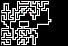
A circle-free graph can be sorted topologically with the depth first search in runtime . ${\ displaystyle {\ mathcal {O}} (\ vert V \ vert + \ vert E \ vert)}$

Solving puzzles with just one solution, e.g. B. mazes . Depth-first search can be adjusted to find all solutions to a maze by including only nodes on the current path in the visited set.
A random depth-first search can be used to create a maze .

literature

Stuart Russell, Peter Norvig : Artificial Intelligence: A Modern Approach . 2nd Edition. Prentice Hall, 2002.
Sven Oliver Krumke, Hartmut Noltemeier: Graph theory concepts and algorithms . 3. Edition. Springer Vieweg, 2012, ISBN 978-3-8348-1849-2

Web links

Commons : Depth-first search - collection of images, videos and audio files

Wikibooks: Depth-First Search - Implementations in the Algorithm Collection

Clear explanation of depth-first search using the example of a labyrinth

Individual evidence

↑ Volker Turau: Algorithmic Graph Theory . 3. Edition. Oldenbourg Wissenschaftsverlag, Munich 2009, ISBN 978-3-486-59057-9 , p. 94-98 .
↑ Thomas H. Cormen, Charles Leiserson , Ronald L. Rivest , Clifford Stein: Algorithmen - An Introduction . 3. Edition. Oldenbourg Wissenschaftsverlag, Munich 2010, ISBN 978-3-486-59002-9 , p. 613-622 .
↑ Thomas Ottmann, Peter Widmayer: Algorithms and Data Structures . 5th edition. Spektrum Akademischer Verlag, Heidelberg 2012, ISBN 978-3-8274-2803-5 , p. 589-668 .
↑ John Hopcroft, Robert E. Tarjan: Efficient planarity testing . In: Journal of the Association for Computing Machinery . 21, No. 4, 1974, pp. 549-568. doi : 10.1145 / 321850.321852 .
↑ H. de Fraysseix, P. Ossona de Mendez, P. Rosenstiehl: Trémaux Trees and Planarity . In: International Journal of Foundations of Computer Science . 17, No. 5, 2006, pp. 1017-1030. arxiv : math / 0610935 . doi : 10.1142 / S0129054106004248 .
↑ ^a ^b Sven Oliver Krumke, Hartmut Noltemeier: Graph Theoretical Concepts and Algorithms . 3. Edition. Springer Vieweg, Wiesbaden 2012, ISBN 978-3-8348-1849-2 , p. 152-157 .

[1] Volker Turau: Algorithmic Graph Theory . 3. Edition. Oldenbourg Wissenschaftsverlag, Munich 2009, ISBN 978-3-486-59057-9 , p. 94-98 .

[2] Thomas H. Cormen, Charles Leiserson , Ronald L. Rivest , Clifford Stein: Algorithmen - An Introduction . 3. Edition. Oldenbourg Wissenschaftsverlag, Munich 2010, ISBN 978-3-486-59002-9 , p. 613-622 .

[3] Thomas Ottmann, Peter Widmayer: Algorithms and Data Structures . 5th edition. Spektrum Akademischer Verlag, Heidelberg 2012, ISBN 978-3-8274-2803-5 , p. 589-668 .

[4] John Hopcroft, Robert E. Tarjan: Efficient planarity testing . In: Journal of the Association for Computing Machinery . 21, No. 4, 1974, pp. 549-568. doi : 10.1145 / 321850.321852 .

[5] H. de Fraysseix, P. Ossona de Mendez, P. Rosenstiehl: Trémaux Trees and Planarity . In: International Journal of Foundations of Computer Science . 17, No. 5, 2006, pp. 1017-1030. arxiv : math / 0610935 . doi : 10.1142 / S0129054106004248 .

[Krumke2012-6] Sven Oliver Krumke, Hartmut Noltemeier: Graph Theoretical Concepts and Algorithms . 3. Edition. Springer Vieweg, Wiesbaden 2012, ISBN 978-3-8348-1849-2 , p. 152-157 .