The Biot-Savart law describes the magnetic field of moving charges. It establishes a connection between the magnetic field strength and the electrical current density and allows the calculation of spatial magnetic field strength distributions based on the knowledge of the spatial current distributions. Here the law is treated as the relationship between magnetic flux density and electric current density .


In a vacuum and in magnetically linear and isotropic materials, there is a connection between the magnetic flux density and the magnetic field strength and the magnetic conductivity as a constant proportionality factor. In the general case (e.g. in the case of magnets), on the other hand, the magnetic conductivity can be a function of the magnetic field strength or the spatial orientation, which can result in significantly more complicated and analytically no longer representable relationships.


This law was named after the two French mathematicians Jean-Baptiste Biot and Félix Savart , who formulated it in 1820. In addition to Ampère's law, it represents one of the basic laws of magnetostatics , a branch of electrodynamics .
formulation
A current conductor with the infinitesimal length element at the location , through which a current flows, generates the magnetic flux density at the location (using the cross product ):


The entire magnetic flux density is obtained by adding up all existing infinitesimal components, i.e. by integrating. The resulting path integral can be calculated using

transform into a volume integral, where is the electrical current density . This gives the integral form of Biot-Savart's law:

These two formulas are similar (with currents instead of charges) to Coulomb's law , which describes the shape of the electric field as a function of a charge distribution.
In the two above formulas it was neglected that the current conductors have a finite cross-section. In many real applications, this is actually irrelevant compared to the expansion of the magnetic field. Another inaccuracy is that the contribution of a charge in one place to the magnetic field in another place spreads at the speed of light . The corresponding retardation effect is not taken into account in the Biot-Savart law. It is therefore only strictly valid for stationary currents and a good approximation for point charges, provided that their speed is small compared to the speed of light.
Derivation from the Maxwell equations
In the following, retardation effects are neglected and the time-constant case in the form of magnetostatics is considered. The Poisson's equation for the vector potential then follows from the Maxwell equations 

with the following solution:

It follows for the magnetic flux density:

With the help of the formulas for the application of the rotation operator to a product of a scalar function and a vector function and of


the end result follows if one takes into account that in the integral only acts on the variable and not on . It is often more advantageous to calculate the vector potential and from this the magnetic flux density.

The same result is obtained by using the Helmholtz decomposition and the Maxwell equations for the static case.
application
Circular conductor loop
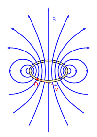
Magnetic field in a current loop
The magnitude of the magnetic flux density of a circular, counterclockwise flowed conductor loop can be specified with the help of the Biot-Savart law on the symmetry axis perpendicular to the conductor loop:

Here is the radius of the conductor loop lying in the plane . The field is directed in the direction.


Through the substitution

one gets from it

In this case , the field of the conductor loop can be treated as a dipole field : For example, for points on the -axis it shows a -dependence for large distances (large ) :


with the magnetic (dipole) moment (current × area of the conductor loop).

Straight line cable
Cylindrical coordinates are suitable for calculating the flux density of a straight line conductor of length . The origin of the coordinate system is placed in the middle of the line cable parallel to the axis. The current density of the line conductor is then with the delta distribution and the Heaviside function . This simplifies the volume integral of Biot-Savart's law to a simple integral over and the vector potential follows as:


In the case of the line conductor, it is easier to first form the rotation and then integrate it. Since the vector potential has only one component and this does not depend on, this is

-
 .
.
The substitution provides with then


-
 .
.

-Field of a straight conductor
The case of an infinitely long straight line conductor results from the borderline case of the straight conductor with .


The magnetic flux density only depends on the radial distance between the point and the conductor, since the translation symmetry means that the dependence on must disappear.
Frame coil

Dependencies for calculating the frame coil
After the round coil, the frame coil (with turns) is the most frequently used variant. The formula for the magnetic field in the center can be derived from the formula for the line conductor by treating the straight sections of the coil as a line conductor.


With


For the magnetic field on the axis, at a great distance from the coil, results


so again a dependency as with the dipole. With a magnetic moment :


Point loading at constant speed
In the case of a point charge that moves at constant speed according to Maxwell's equations, the equations apply to the electric and magnetic fields


-
 or reshaped

where is the unit vector pointing from the instantaneous (non-retarded) position of the particle to the point at which the field is measured and the angle between and .


In this case , the electric and magnetic fields can be approximated as follows:


These equations are called (because of the analogy with the “normal” Biot – Savart law) “Biot – Savart law for a point charge”. They were first derived by Oliver Heaviside in 1888.
See also
literature
Remarks
-
↑ Article on Félix Savart. At: www-groups.dcs.st-and.ac.uk. Retrieved May 21, 2016.
-
↑ a b David J. Griffiths: Introduction to Electrodynamics (3rd ed.) . Prentice Hall, 1998, ISBN 0-13-805326-X , pp. 222-224, 435-440.
-
^ Magnetic Field From a Moving Point Charge . Archived from the original on June 19, 2009. Retrieved September 30, 2009.


