Hidden Markov Model

The Hidden Markov Model , short HMM ( German concealed Markowmodell , or hidden Markowmodell ) is a stochastic model in which a system by a Markov chain - named after the Russian mathematician AA Markov is modeled with unobserved states -. An HMM can thus be viewed as the simplest special case of a dynamic Bayesian network .

Modeling as a Markov chain means that the system changes from one state to another in a random manner, with the transition probabilities only depending on the current state, but not on the previous states. It is also assumed that the transition probabilities are constant over time. With an HMM, however, the states themselves are not observed from the outside; they are hidden (engl. hidden , see also latent variable model ). Instead, each of these internal states is assigned observable output symbols (so-called emissions ) that occur with certain probabilities depending on the state. The task is mostly to come from the observed sequence of emissions to probabilistic statements about the hidden states.

Since the Markov models are closely related to the state space models used in control engineering, care must be taken to ensure that the term “observe” is not confused with the control engineering term “ observability ”, which Rudolf Kálmán introduced in 1960 and describes an independent system property . “Observing” in the sense of the Markov models is referred to as “measuring” in control engineering. The “unobserved” or “hidden” states in the sense of the Markov theory can very well be observable in the sense of control engineering, but need not be.

Important areas of application are voice and handwriting recognition , computational linguistics and bioinformatics , spam filter , gesture recognition in the man-machine communication , physical chemistry and psychology .

Markov approach

Given are two time-discrete random processes and , of which only the last can be observed. It is intended to draw conclusions about the course of the first process; this requires a mathematical model that relates the two processes to one another. ${\displaystyle \{X_{t}\}_{t\in \mathbb {N} }}$ ${\displaystyle \{Y_{t}\}_{t\in \mathbb {N} }}$

The approach described here is characterized by the following two assumptions:

1. Markov property

The current value of the first process depends entirely on its last value:

${\displaystyle \forall t\in \mathbb {N} \colon P(X_{t}=x_{t}|X_{1}=x_{1};\ldots ;X_{t-1}=x_{t-1};Y_{1}=y_{1};\ldots ;Y_{t-1}=y_{t-1})=P(X_{t}=x_{t}|X_{t-1}=x_{t-1})}$.

2. Markov property

The current value of the second process depends exclusively on the current value of the first:

${\displaystyle \forall t\in \mathbb {N} \colon P(Y_{t}=y_{t}|X_{1}=x_{1};\ldots ;X_{t}=x_{t};Y_{1}=y_{1};\ldots ;Y_{t-1}=y_{t-1})=P(Y_{t}=y_{t}|X_{t}=x_{t})}$.

If both processes now have a finite set of values, the model obtained in this way can be understood as a probabilistic automaton , more precisely as a Markov chain . It is also said that it is a Markov trial . Based on the linguistic usage in theoretical computer science - in particular the automaton theory and the theory of formal languages - the values ​​of the first process are called states and those of the second are emissions or outputs . ${\displaystyle \{X_{t}\}}$

definition

Parameters of a Hidden Markov Model (example)
x - (hidden) states
y - possible observations (emissions)
a - transition probabilities
b - emission probabilities

A hidden Markov model is a 5- tuple with: ${\displaystyle \lambda =(S;V;A;B;\pi )}$

• ${\displaystyle S=\{s_{1};\dotsc ;s_{n}\}}$the set of all states , these are the possible values ​​of the random variables , ${\displaystyle X_{t}}$
• ${\displaystyle V=\{v_{1};\dotsc ;v_{m}\}}$the alphabet of possible observations - the emissions of , ${\displaystyle Y_{t}}$
• ${\displaystyle A\in \mathbb {R} ^{n\times n}}$the transition matrix between the states are in each case the probability that the state in the state is changed, ${\displaystyle a_{ij}=P(X_{t}=s_{j}|X_{t-1}=s_{i})}$ ${\displaystyle s_{i}}$ ${\displaystyle s_{j}}$
• ${\displaystyle B\in \mathbb {R} ^{n\times m}}$the observation matrix, which indicate the probability of making the observation in the state , as well as ${\displaystyle b_{ij}=P(Y_{t}=v_{j}|X_{t}=s_{i})}$ ${\displaystyle s_{i}}$ ${\displaystyle v_{j}}$
• ${\displaystyle \pi \in \mathbb {R} ^{n}}$the initial distribution, is the probability that the initial state is. ${\displaystyle \pi _{i}=P(X_{1}=s_{i})}$ ${\displaystyle s_{i}}$

An HMM is called stationary (or also time-invariant ) if the transition and emission probabilities do not change over time. This assumption often makes sense because the modeled laws of nature are also constant.

illustration

Temporal development of an HMM

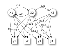
The picture shows the general architecture of an instantiated HMM. Each oval is the representation of a random variable or that any values or can take. The first random variable is the hidden state of the HMM at the time , the second is the observation at this time. The arrows in the trellis diagram indicate a conditional dependency . ${\displaystyle x(t)}$ ${\displaystyle y(t)}$ ${\displaystyle S}$ ${\displaystyle V}$ ${\displaystyle t}$

In the diagram you can see that the state of the hidden variable only depends on the state of the variable ; earlier values ​​have no further influence. Therefore the model is a 1st order Markov model. If higher orders are required, these can always be traced back to the 1st order by inserting new hidden states. The value of further depends solely on. ${\displaystyle x(t)}$ ${\displaystyle x(t-1)}$ ${\displaystyle y(t)}$ ${\displaystyle x(t)}$

example

Prisoner in the dungeon

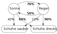
A prisoner in the dungeon wants to find out the current weather. He knows that a sunny day is 70% followed by a rainy day and that a rainy day is 50% followed by a sunny day. If he also knows that the guards 'shoes are 90% dirty in the rain, but only 60% dirty in sunny weather, he can draw conclusions about the weather by observing the guards' shoes (i.e. he can compare the probability of rainy weather estimate sunny weather). Here, the actually existing but invisible weather forms the hidden state to be determined, the percentages 70% and 50% are training data of the model (determined over longer periods of time), and the actually observable states are in the respective appearance of the shoes.

DNA sequence: find CpG islands

The HMM can be used to study DNA sequences with bioinformatic methods. For example, CpG islands can be found in a DNA sequence. These are areas of a DNS -Einzelstrangs having an increased content of consecutive cytosine - and guanine - nucleic bases . The DNA sequence represents the observation, the characters of which form the output alphabet. In the simplest case, the HMM has two hidden states, namely CpG island and non-CpG island . These two states differ in their output distribution, so that the CpG island state is more likely to output characters and . ${\displaystyle V=\{A,C,G,T\}}$ ${\displaystyle C}$ ${\displaystyle G}$

voice recognition

In the automatic speech recognition with HMM, the spoken sounds are interpreted as hidden states and the actually audible tones as emissions.

Problems

There are several fundamental problems associated with HMMs.

Determine the model size

The observable emissions are given . It must be clarified which model properties - in particular which orthogonal dimensionality - allow the conclusion about the not directly observable states and at the same time allow a meaningful calculability . In particular, it has to be decided which running time may be required for the model calculations in order to maintain the usability of the estimates. ${\displaystyle V}$

implementation

The calculation of the estimated values ​​of the unobservable states from the observable output sequences must consider the achievable numerical accuracies. Criteria for classifying statistical significance must also be implemented. When using an HMM for a specific feature vector, the significance determines the probability of a correct or incorrect model hypothesis and its information content ( entropy , conditional entropy ) or its information quality .

Filter

An HMM and an observation sequence of length are given . Wanted is the probability that the current hidden state for the last time just is. An efficient method for solving the filtering problem is the forward algorithm . ${\displaystyle \lambda }$ ${\displaystyle {\boldsymbol {o}}\in V^{*}}$ ${\displaystyle T}$ ${\displaystyle P(X_{T}=s_{i}|{\boldsymbol {o}};\lambda )}$ ${\displaystyle T}$ ${\displaystyle s_{i}}$

Prediction / prediction

Again, an HMM and the observation sequence and a . What we are looking for is probability , i.e. the probability that the HMM is in the state at the time if the relevant output was observed. Prediction is, so to speak, repeated filtering without new observations and can also be easily calculated using the forward algorithm . ${\displaystyle \lambda }$ ${\displaystyle {\boldsymbol {o}}}$ ${\displaystyle \delta \geq 1}$ ${\displaystyle P(X_{T+\delta }=s_{i}|{\boldsymbol {o}};\lambda )}$ ${\displaystyle T+\delta }$ ${\displaystyle s_{i}}$

Smooth

Be again , and given a. We are looking for the probability , i.e. the probability that the model was in a certain state at an earlier point in time, under the condition that it was observed. This probability can be calculated efficiently with the help of the forward-backward algorithm . ${\displaystyle \lambda }$ ${\displaystyle {\boldsymbol {o}}}$ ${\displaystyle \delta }$ ${\displaystyle P(X_{T-\delta }=s_{i}|{\boldsymbol {o}};\lambda )}$ ${\displaystyle {\boldsymbol {o}}}$

Decoding

Be given again as well . The aim is to determine the most likely sequence of states that a given output sequence could have generated. This problem can be solved efficiently with the Viterbi algorithm . ${\displaystyle \lambda }$ ${\displaystyle {\boldsymbol {o}}}$ ${\displaystyle S^{*}}$

Learning problem

Only the output sequence is given . The aim is to determine the parameters of an HMM that are most likely to generate the output sequence. This can be solved with the help of the Baum-Welch algorithm . ${\displaystyle {\boldsymbol {o}}}$

Interpretation problem

Only the possible expenses are given . The states in the model system and the corresponding effects in the real system are to be identified, which describe the state set of the model. To do this, the significance of the individual emissions must be determined in advance . ${\displaystyle V}$ ${\displaystyle S}$

application areas

HMMs are often used in pattern recognition when processing sequential data, for example in physical measurement series , recorded speech signals or protein sequences . For this purpose, the models are constructed in such a way that the hidden states correspond to semantic units (e.g. phonemes in speech recognition ) that are to be recognized in the sequential data (e.g. short-term spectra of the speech signal). Another application is to find, for a given HMM, by searching a random sample of sequential data, those sequences that could very likely have been generated by this HMM. For example, an HMM that has been trained with representatives of a protein family can be used to find additional representatives of this family in large protein databases.

history

Hidden Markov models were first published by Leonard E. Baum and other authors in the second half of the 1960s. One of the first applications from the mid-1970s was speech recognition. HMMs have been used for the analysis of nucleotide and protein sequences since the mid-1980s and have been an integral part of bioinformatics ever since .

literature

• R. Merkl, S. Waack: Interactive bioinformatics. Wiley-VCH, 2002, ISBN 3-527-30662-5 .
• GA Fink: Pattern recognition with Markov models: theory, practice, areas of application. Teubner, 2003, ISBN 3-519-00453-4 .
• Kai-Fu Lee, Hsiao-Wuen Hon: Speaker-Independent Phone Recognition Using Hidden Markov Models . IEEE Transactions on Accoustics, Speech and Signal Processing, No. 37 . IEEE, November 1989, pp. 1641-1648 (English, IEEE No. 8930533, 0096-3518 / 89 / 1100-1641).

Web links

• Rv Handel, July 28, 2008: Hidden Markov Models (PDF; 900 kB; 123 pages) Lecture Notes Princeton University July 2008, accessed on February 24, 2019.
• EG Schukat-Talamazzini, December 7th, 2018: Special pattern analysis systems (PDF; 1.3 MB; 17 pages) Lecture in WS 2018 at the University of Jena. Cape. 5, accessed February 24, 2019.
• HMM R package for modeling and analyzing hidden Markov models, which is freely available under GPL2
• http://code.google.com/p/jahmm/ HMM Java library which is available under the new BSD license.
• http://www.ghmm.org HMM C library which is freely available under the LGPL

Individual evidence

1. ^ S. Schmid, Dissertation, Technical University of Munich, Munich, 2017. Single Protein Dynamics at Steady State Quantified from FRET Time Traces
2. ^ LR Rabiner: A Tutorial on Hidden Markov Models and Selected Applications in Speech Recognition. (PDF; 2.2 MB; 30 pages) Proceedings of the IEEE, Volume 77, No. 2, pp. 257-286, 1989.
3. ↑ P. Blunsom, August 19, 2004: Hidden Markov Models (PDF; 237 kB; 7 pages), archive.org, accessed on February 21, 2019.
4. ↑ SP Chatzis: A Variational Bayesian Methodology for Hidden Markov Models .