Convective coordinates

Coordinate lines applied to a body follow the deformations of the body

Convective coordinates are curvilinear coordinates that are tied to a carrier and are carried along by all transformations that the carrier experiences, hence the term convective. In continuum mechanics , convective coordinates result naturally when the coordinate lines are solid lines that follow all movements and deformations of the body. You can imagine a coordinate network painted on a rubber skin, which is then stretched and takes the coordinate network with it, see figure on the right.

Convective coordinate systems are of practical importance in the kinematics of slim structures ( bars , beams ) and thin-walled structures ( shells and membranes ), where the stresses and strains parallel to the preferred directions of the structure are of interest. In addition, preferred material directions of non-isotropic materials, such as. B. of wood, or advection-diffusion problems (e.g. the spread of pollutants in the atmosphere or in the groundwater) can be described in convective coordinates. In the kinematics of deformable bodies, the tensors used in continuum mechanics , expressed in convective coordinates, have particularly simple representations.

definition

Configurations and Convective Coordinates

A deformable body is considered as in the picture, which is mapped into a Euclidean vector space by means of configurations . The convective coordinates of a material point are assigned by the reference configuration. For every particle of a body its convective coordinates are given by: ${\displaystyle \mathbb {V} ^{3}}$ ${\displaystyle P}$ ${\displaystyle \kappa _{R}(P)}$ ${\displaystyle P}$ ${\displaystyle K}$

${\displaystyle {\begin{array}{llll}\kappa _{R}:&K&\rightarrow &V_{R}\subset \mathbb {V} ^{3}\\&P&\mapsto &{\vec {\Theta }}=(\Theta _{1},\Theta _{2},\Theta _{3})\end{array}}}$

This assignment is independent of the chosen reference system of the observer, of the time and of the physical space of our perception. For the square body in the picture, e.g. B. the unit square as the image area. is unambiguous (bijective) , so that the particle can also be named. Because the coordinates are tied to the particle, they are carried along with every movement of the particle. ${\displaystyle V_{R}=[0,1]^{2}}$ ${\displaystyle \kappa _{R}}$ ${\displaystyle {\vec {\Theta }}}$ ${\displaystyle P}$ ${\displaystyle {\vec {\Theta }}}$

Tangent and gradient vectors

Coordinate line of with tangent vector and gradient vector in the point ${\displaystyle \Theta _{1}}$ ${\displaystyle {\vec {G}}_{1}}$ ${\displaystyle {\vec {G}}^{1}}$ ${\displaystyle {\vec {X}}}$

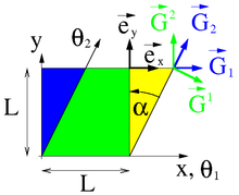
The covariant tangent vectors and on material coordinate lines (black) in the initial or current configuration span tangential spaces (yellow). The contravariant basis vectors and span cotangent spaces (not shown) ${\displaystyle {\vec {G}}_{1,2,3}}$ ${\displaystyle {\vec {g}}_{1,2,3}}$ ${\displaystyle \color {blue}{\vec {G}}^{1,2,3}}$ ${\displaystyle \color {blue}{\vec {g}}^{1,2,3}}$

The movement function describes the movement of the particle through the space of our perception and provides us with an object of our perception because these positions have been taken by the body once. The movement starts at a certain point in time when the body is in the initial configuration. The function ${\displaystyle {\vec {x}}={\vec {\chi }}_{t}({\vec {\Theta }},t)\in \mathbb {V} ^{3}}$ ${\displaystyle {\vec {\Theta }}}$ ${\displaystyle t_{0}}$

${\displaystyle {\vec {\chi }}_{0}({\vec {\Theta }}):={\vec {\chi }}_{t}({\vec {\Theta }},t_{0})={\vec {X}}=\sum _{i=1}^{3}X_{i}{\vec {e}}_{i}}$

assigns the coordinates uniquely (bijective) to a point in space that the particle occupied at the time . The vector has material coordinates with respect to the standard base . Because of the bijectivity can ${\displaystyle {\vec {\Theta }}}$ ${\displaystyle {\vec {X}}}$ ${\displaystyle t_{0}}$ ${\displaystyle {\vec {X}}}$ ${\displaystyle X_{1,2,3}}$ ${\displaystyle {\vec {e}}_{1,2,3}}$

${\displaystyle {\vec {X}}=:{\vec {\chi }}_{0}({\vec {\Theta }})\quad \Leftrightarrow \quad {\vec {\Theta }}=:{\vec {\chi }}_{0}^{-1}({\vec {X}})}$

to be written. If only one coordinate varies in the vector , then a material coordinate line follows, which in general is a curve in space, see figure above on the right. The tangent vectors ${\displaystyle {\vec {\Theta }}}$ ${\displaystyle \Theta _{i}}$ ${\displaystyle {\vec {\chi }}_{0}({\vec {\Theta }})}$

${\displaystyle {\vec {G}}_{i}={\frac {\mathrm {d} {\vec {\chi }}_{0}}{\mathrm {d} \Theta _{i}}}=\sum _{j=1}^{3}{\frac {\mathrm {d} \chi _{0j}}{\mathrm {d} \Theta _{i}}}{\vec {e}}_{j}}$

on these curves are called covariant basis vectors of the curvilinear coordinate system. The direction in which the coordinate changes the most are the gradients ${\displaystyle \Theta _{i}}$

${\displaystyle {\vec {G}}^{i}={\frac {\mathrm {d} \Theta _{i}}{\mathrm {d} {\vec {X}}}}:=\mathrm {GRAD} (\Theta _{i})=\sum _{j=1}^{3}{\frac {\mathrm {d} \Theta _{i}}{\mathrm {d} X_{j}}}{\vec {e}}_{j}}$

which represent the contravariant basis vectors in a material point. Because of ${\displaystyle {\vec {G}}^{i}}$

${\displaystyle {\begin{aligned}{\frac {\mathrm {d} \Theta _{i}}{\mathrm {d} \Theta _{j}}}=&\sum _{k=1}^{3}{\frac {\mathrm {d} \Theta _{i}}{\mathrm {d} X_{k}}}\cdot {\frac {\mathrm {d} X_{k}}{\mathrm {d} \Theta _{j}}}=\sum _{k,l=1}^{3}{\frac {\mathrm {d} \Theta _{i}}{\mathrm {d} X_{k}}}{\vec {e}}_{k}\cdot {\frac {\mathrm {d} X_{l}}{\mathrm {d} \Theta _{j}}}{\vec {e}}_{l}\\=&{\vec {G}}^{i}\cdot {\vec {G}}_{j}=\left\{{\begin{array}{lll}1&\mathrm {falls} &i=j\\0&\mathrm {sonst} &\end{array}}\right.\end{aligned}}}$

the co- and contravariant basis vectors are dual to each other and the contravariant basis vectors can be from

${\displaystyle {\begin{aligned}\mathbf {J} =&\sum _{i,j=1}^{3}{\frac {\mathrm {d} \chi _{0i}}{\mathrm {d} \Theta _{j}}}{\vec {e}}_{i}\otimes {\vec {e}}_{j}=\sum _{j=1}^{3}{\vec {G}}_{j}\otimes {\vec {e}}_{j}\\\rightarrow \mathbf {J} ^{-1}=&\displaystyle \left(\sum _{j=1}^{3}{\vec {G}}_{j}\otimes {\vec {e}}_{j}\right)^{-1}=\sum _{i=1}^{3}{\vec {e}}_{i}\otimes {\vec {G}}^{i}\end{aligned}}}$

be calculated. The dyadic product " " was used in it. ${\displaystyle \otimes }$

The deformation gradient J operating between the reference configuration and the initial configuration contains the covariant basis vectors in the columns and the contravariant basis vectors are found in the rows of its inverse . ${\displaystyle {\vec {G}}_{i}}$ ${\displaystyle {\vec {G}}^{i}}$ ${\displaystyle \mathbf {J} ^{-1}}$

The co- and contravariant basis vectors are only used locally (in the tangential spaces ) in the point as a basis system for vector and tensor fields, but not for position vectors: The covariant basis vectors form a basis of the tangent space and the contravariant basis vectors form a basis of the cotangent space in the point , see figure below on the right. ${\displaystyle {\vec {X}}}$ ${\displaystyle {\vec {G}}_{i}}$ ${\displaystyle T_{\vec {X}}\mathbb {V} ^{3}}$ ${\displaystyle {\vec {G}}^{i}}$ ${\displaystyle T_{\vec {X}}^{\ast }\mathbb {V} ^{3}}$ ${\displaystyle {\vec {X}}}$

In the course of the movement, a set of covariant basis vectors and contravariant basis vectors are created at each point and at each point in time , which are the tangents or gradients of the material coordinate lines in the deformed body at the time . They are therefore bases of the tangent spaces or . ${\displaystyle t>t_{0}}$ ${\displaystyle {\vec {g}}_{i}}$ ${\displaystyle {\vec {g}}^{i}}$ ${\displaystyle t}$ ${\displaystyle T_{\vec {x}}\mathbb {V} ^{3}}$ ${\displaystyle T_{\vec {x}}^{\ast }\mathbb {V} ^{3}}$

Differential operators and Nabla operators

→ Main article : Nabla operator

The differential operators gradient (grad), divergence (div) and rotation (red) from vector analysis can be defined with the Nabla operator . In convective coordinates, the Nabla operator in Lagrange's representation has the form: ${\displaystyle \nabla }$

${\displaystyle \nabla _{0}:=\sum _{i=1}^{3}{\vec {G}}^{i}{\frac {\partial }{\partial \Theta _{i}}}}$

The gradients of scalar and vector fields are represented with it as follows:

Scalar field	${\displaystyle \mathrm {GRAD} (\phi ):=\nabla _{0}\,\phi =\sum _{i=1}^{3}{\frac {\partial \phi }{\partial \Theta _{i}}}{\vec {G}}^{i}=:{\frac {\partial \phi }{\partial {\vec {X}}}}}$
Vector field	${\displaystyle \mathrm {GRAD} ({\vec {v}}):=(\nabla _{0}\otimes {\vec {v}})^{\top }=\sum _{i=1}^{3}{\frac {\partial {\vec {v}}}{\partial {\Theta }_{i}}}\otimes {\vec {G}}^{i}=:{\frac {\partial {\vec {v}}}{\partial {\vec {X}}}}}$

The divergences are obtained from the scalar product with : ${\displaystyle \nabla _{0}}$

Vector field	${\displaystyle \mathrm {DIV} ({\vec {v}}):=\nabla _{0}\cdot {\vec {v}}=\sum _{i=1}^{3}{\frac {\partial {\vec {v}}}{\partial \Theta _{i}}}\cdot {\vec {G}}^{i}=\mathrm {Sp} \left({\frac {\partial {\vec {v}}}{\partial {\vec {X}}}}\right)}$
Tensor field	${\displaystyle \mathrm {DIV} (\mathbf {T} ):=\nabla _{0}\cdot \mathbf {T} =\sum _{i=1}^{3}{\vec {G}}^{i}\cdot {\frac {\partial \mathbf {T} }{\partial \Theta _{i}}}}$

The operator Sp forms the track . The rotation of a vector field arises with the cross product :

${\displaystyle \mathrm {ROT} ({\vec {v}}):=\nabla _{0}\times {\vec {v}}=\sum _{i=1}^{3}{\vec {G}}^{i}\times {\frac {\partial {\vec {v}}}{\partial \Theta }}_{i}}$

Corresponding operators , and for fields in Euler's representation , the Nabla operator provides ${\displaystyle \mathrm {div} }$ ${\displaystyle \mathrm {grad} }$ ${\displaystyle \mathrm {rot} }$

${\displaystyle \nabla _{t}:=\sum _{i=1}^{3}{\vec {g}}^{i}{\frac {\partial }{\partial \Theta _{i}}}}$

The unit tensor

→ Main article : Unit tensor

The unit tensor maps each vector onto itself. With regard to the co- and contravariant basis vectors, his representations are: ${\displaystyle \mathbf {1} }$

${\displaystyle \mathbf {1} =\sum _{i=1}^{3}{\vec {G}}^{i}\otimes {\vec {G}}_{i}=\sum _{i=1}^{3}{\vec {G}}_{i}\otimes {\vec {G}}^{i}=\sum _{i,j=1}^{3}G_{ij}{\vec {G}}^{i}\otimes {\vec {G}}^{j}=\sum _{i,j=1}^{3}G^{ij}{\vec {G}}_{i}\otimes {\vec {G}}_{j}}$

The scalar products of the covariant basis vectors

${\displaystyle G_{ij}={\vec {G}}_{i}\cdot {\vec {G}}_{j}}$

are called covariant metric coefficients (of the tangent space ). The scalar products of the contravariant basis vectors are correspondingly ${\displaystyle T_{\vec {X}}\mathbb {V} ^{3}}$

${\displaystyle G^{ij}={\vec {G}}^{i}\cdot {\vec {G}}^{j}}$

contravariant metric coefficients (of the cotangent space ). ${\displaystyle T_{\vec {X}}^{\ast }\mathbb {V} ^{3}}$

In Euler's approach, the same applies

${\displaystyle \mathbf {1} =\sum _{i=1}^{3}{\vec {g}}^{i}\otimes {\vec {g}}_{i}=\sum _{i=1}^{3}{\vec {g}}_{i}\otimes {\vec {g}}^{i}=\sum _{i,j=1}^{3}g_{ij}{\vec {g}}^{i}\otimes {\vec {g}}^{j}=\sum _{i,j=1}^{3}g^{ij}{\vec {g}}_{i}\otimes {\vec {g}}_{j}}$

with the co- and contravariant metric coefficients or (of the tangential space or cotangential space ). ${\displaystyle g_{ij}={\vec {g}}_{i}\cdot {\vec {g}}_{j}}$ ${\displaystyle g^{ij}={\vec {g}}^{i}\cdot {\vec {g}}^{j}}$ ${\displaystyle T_{\vec {x}}\mathbb {V} ^{3}}$ ${\displaystyle T_{\vec {x}}^{\ast }\mathbb {V} ^{3}}$

Deformation gradient

→ Main article : Deformation gradient

Expressed in convective coordinates, the deformation gradient takes on a particularly simple form. According to its definition, the deformation gradient maps the tangent vectors on material lines in the initial configuration to those in the current configuration and these tangent vectors are precisely the covariant base vectors or . So is ${\displaystyle \mathbf {F} }$ ${\displaystyle {\vec {G}}_{i}}$ ${\displaystyle {\vec {g}}_{i}}$

${\displaystyle {\vec {g}}_{i}=\mathbf {F} \cdot {\vec {G}}_{i}\quad \Leftrightarrow \quad \mathbf {F} =\sum _{i=1}^{3}{\vec {g}}_{i}\otimes {\vec {G}}^{i}}$

This also results from the derivation of the motion function  : ${\displaystyle {\vec {x}}={\vec {\chi }}({\vec {X}},t)={\vec {\chi }}_{t}({\vec {\Theta }},t)}$

${\displaystyle \mathbf {F} =\mathrm {GRAD} \;{\vec {\chi }}({\vec {X}},t)={\vec {\chi }}_{t}\otimes \nabla _{0}=\sum _{i=1}^{3}{\frac {\mathrm {d} {\vec {\chi }}_{t}}{\mathrm {d} \Theta _{i}}}\otimes {\vec {G}}^{i}=\sum _{i=1}^{3}{\vec {g}}_{i}\otimes {\vec {G}}^{i}}$

In this representation you can also immediately with

${\displaystyle \mathbf {F} ^{-1}=\sum _{i=1}^{3}{\vec {G}}_{i}\otimes {\vec {g}}^{i}}$

specify the inverse of the deformation gradient. The transposed inverse deformation gradient maps the contravariant basis vectors to one another:

${\displaystyle \mathbf {F} ^{\top -1}=\sum _{i=1}^{3}{\vec {g}}^{i}\otimes {\vec {G}}_{i}\quad \Leftrightarrow \quad {\vec {g}}^{i}=\mathbf {F} ^{\top -1}\cdot {\vec {G}}^{i}}$

Spatial velocity gradient

→ Main article : Velocity gradient

The material time derivative of the deformation gradient is the material velocity gradient

${\displaystyle {\dot {\mathbf {F} }}=\sum _{i=1}^{3}{\dot {\vec {g}}}_{i}\otimes {\vec {G}}^{i}}$

because the initial configuration does not depend on the time and that also applies to the basis vectors and . The spatial velocity gradient is given the simple form in convective coordinates ${\displaystyle {\vec {G}}_{i}}$ ${\displaystyle {\vec {G}}^{i}}$ ${\displaystyle \mathbf {l} }$

${\displaystyle \mathbf {l} =\mathrm {grad} ({\vec {v}}({\vec {x}},t))={\dot {\mathbf {F} }}\cdot \mathbf {F} ^{-1}=\sum _{i=1}^{3}{\dot {\vec {g}}}_{i}\otimes {\vec {g}}^{i}=-\sum _{i=1}^{3}{\vec {g}}_{i}\otimes {\dot {\vec {g}}}^{i}}$

where is the velocity of a particle in place at time . The spatial velocity gradient transforms the basis vectors into their rates: ${\displaystyle {\vec {v}}({\vec {x}},t)}$ ${\displaystyle {\vec {x}}}$ ${\displaystyle t}$

${\displaystyle {\dot {\vec {g}}}_{i}=\mathbf {l} \cdot {\vec {g}}_{i}}$   and    ${\displaystyle {\dot {\vec {g}}}^{i}=-\mathbf {l} ^{\top }\cdot {\vec {g}}^{i}}$

Stretch, strain and stress tensors

The following tensors appear in continuum mechanics . Their representation in convective coordinates is compiled in the table.

Surname	Representation in convective coordinates
Deformation gradient	${\displaystyle \mathbf {F} =\sum _{i=1}^{3}{\vec {g}}_{i}\otimes {\vec {G}}^{i}}$
Right Cauchy-Green tensor	${\displaystyle \mathbf {C} =\mathbf {F} ^{\top }\cdot \mathbf {F} =\sum _{i,j=1}^{3}g_{ij}{\vec {G}}^{i}\otimes {\vec {G}}^{j}}$
Left Cauchy-Green tensor	${\displaystyle \mathbf {b} =\mathbf {F\cdot F} ^{\top }=\sum _{i,j=1}^{3}G^{ij}{\vec {g}}_{i}\otimes {\vec {g}}_{j}}$
Green-Lagrange strain tensor	${\displaystyle \mathbf {E} ={\frac {1}{2}}(\mathbf {F} ^{\top }\cdot \mathbf {F} -\mathbf {1} )=\sum _{i,j=1}^{3}E_{ij}{\vec {G}}^{i}\otimes {\vec {G}}^{j}}$ With ${\displaystyle E_{ij}={\frac {1}{2}}(g_{ij}-G_{ij})}$
Euler-Almansi strain tensor	${\displaystyle \mathbf {e} ={\frac {1}{2}}(\mathbf {1} -\mathbf {F} ^{\top -1}\cdot \mathbf {F} ^{-1})=\sum _{i,j=1}^{3}E_{ij}{\vec {g}}^{i}\otimes {\vec {g}}^{j}}$
Spatial velocity gradient	${\displaystyle \mathbf {l} =\sum _{i=1}^{3}{\dot {\vec {g}}}_{i}\otimes {\vec {g}}^{i}=-\sum _{i=1}^{3}{\vec {g}}_{i}\otimes {\dot {\vec {g}}}^{i}}$
Spatial strain rate tensor	${\displaystyle \mathbf {d} ={\frac {1}{2}}\sum _{i,j=1}^{3}{\dot {g}}_{ij}{\vec {g}}^{i}\otimes {\vec {g}}^{j}=-{\frac {1}{2}}\sum _{i,j=1}^{3}{\dot {g}}^{ij}{\vec {g}}_{i}\otimes {\vec {g}}_{j}}$
Cauchy's stress tensor	${\displaystyle {\boldsymbol {\sigma }}=\sum _{i,j=1}^{3}\sigma ^{ij}{\vec {g}}_{i}\otimes {\vec {g}}_{j}}$
Weighted Cauchy stress tensor	${\displaystyle \mathbf {S} =\mathrm {det} (\mathbf {F} ){\boldsymbol {\sigma }}=\sum _{i,j=1}^{3}{\tilde {T}}^{ij}{\vec {g}}_{i}\otimes {\vec {g}}_{j}}$
Nominal stress tensor	${\displaystyle \mathbf {N} =\mathrm {det} (\mathbf {F} )\mathbf {F} ^{-1}\cdot {\boldsymbol {\sigma }}=\sum _{i,j=1}^{3}{\tilde {T}}^{ij}{\vec {G}}_{i}\otimes {\vec {g}}_{j}}$
First Piola-Kirchoff stress tensor	${\displaystyle \mathbf {P} =\mathbf {N} ^{\top }=\mathrm {det} (\mathbf {F} ){\boldsymbol {\sigma }}\cdot \mathbf {F} ^{\top -1}=\sum _{i,j=1}^{3}{\tilde {T}}^{ij}{\vec {g}}_{i}\otimes {\vec {G}}_{j}}$
Second Piola-Kirchoff stress tensor	${\displaystyle {\tilde {\mathbf {T} }}=\mathrm {det} (\mathbf {F} )\mathbf {F} ^{-1}\cdot {\boldsymbol {\sigma }}\cdot \mathbf {F} ^{\top -1}=\sum _{i,j=1}^{3}{\tilde {T}}^{ij}{\vec {G}}_{i}\otimes {\vec {G}}_{j}}$

Because the right Cauchy-Green tensor , the Green-Lagrange strain tensor and the Euler-Almansi tensor are formed in their natural form (given here) with the covariant components or , these tensors are usually referred to as covariant tensors . The stress tensors and are accordingly contravariant tensors . ${\displaystyle \mathbf {C} }$ ${\displaystyle \mathbf {E} }$ ${\displaystyle \mathbf {e} }$ ${\displaystyle g_{ij}}$ ${\displaystyle E_{ij}}$ ${\displaystyle {\boldsymbol {\sigma }},\mathbf {S} }$ ${\displaystyle \mathbf {\tilde {T}} }$

Objective time derivations

Objective quantities are those that are perceived in the same way by moving observers. The time derivative of tensors is generally not objective. The convective co- or contravariant Oldroyd derivatives of objective tensors are, however, objective and are written particularly simply in convective coordinates.

The covariate Oldroyd's derivative, e.g. B. of is ${\displaystyle \mathbf {e} =\sum _{i,j=1}^{3}E_{ij}{\vec {g}}^{i}\otimes {\vec {g}}^{j}}$

${\displaystyle {\stackrel {\Delta }{\mathbf {e} }}:={\dot {\mathbf {e} }}+\mathbf {e\cdot l} +\mathbf {l^{\top }\cdot e} =\sum _{i,j=1}^{3}{\dot {E}}_{ij}{\vec {g}}^{i}\otimes {\vec {g}}^{j}}$

The contravariant Oldroyd derivation, e.g. B. von , results similarly: ${\displaystyle \mathbf {S} =\sum _{i,j=1}^{3}{\tilde {T}}^{ij}{\vec {g}}_{i}\otimes {\vec {g}}_{j}}$

${\displaystyle {\stackrel {\nabla }{\mathbf {S} }}:={\dot {\mathbf {S} }}-\mathbf {l\cdot S} -\mathbf {S\cdot l} ^{\top }=\sum _{i,j=1}^{3}{\dot {\tilde {T}}}^{ij}{\vec {g}}_{i}\otimes {\vec {g}}_{j}}$

The terms convective covariant and convective contravariant of the Oldroyd derivatives are derived from this. The matching transformation properties of the covariant tensors are remarkable

${\displaystyle \mathbf {e} =\mathbf {F} ^{\top -1}\cdot \mathbf {E\cdot F} ^{-1}}$    and    ${\displaystyle {\stackrel {\Delta }{\mathbf {e} }}=\mathbf {F} ^{\top -1}\cdot {\dot {\mathbf {E} }}\cdot \mathbf {F} ^{-1}}$

as well as the contravariant tensors

${\displaystyle \mathbf {S} =\mathbf {F} \cdot {\tilde {\mathbf {T} }}\cdot \mathbf {F} ^{\top }}$    and    ${\displaystyle {\stackrel {\nabla }{\mathbf {S} }}=\mathbf {F} \cdot {\dot {\tilde {\mathbf {T} }}}\cdot \mathbf {F} ^{\top }}$

See also the Objective Time Derivatives section in the speed gradient article.

example

Parallelogram in initial and current configuration

A parallelogram with a base and a height and angle of inclination is deformed into a square of the same area, see picture. The unit square is suitable as a reference configuration ${\displaystyle L}$ ${\displaystyle \alpha }$

${\displaystyle \Theta _{1},\Theta _{2}\in [0,L]^{2}\subset \mathbb {R} ^{2}}$

In the initial configuration, the points of the parallelogram have the coordinates:

${\displaystyle {\vec {X}}={\vec {\chi }}_{0}(\Theta _{1},\Theta _{2})=\left({\begin{array}{c}\Theta _{1}+\tan(\alpha )\Theta _{2}\\\Theta _{2}\end{array}}\right)}$

The covariant basis vectors are

${\displaystyle {\vec {G}}_{1}={\frac {\mathrm {d} {\vec {X}}}{\mathrm {d} \Theta _{1}}}=\left({\begin{array}{c}1\\0\end{array}}\right)={\vec {e}}_{x}\,,\;{\vec {G}}_{2}={\frac {\mathrm {d} {\vec {X}}}{\mathrm {d} \Theta _{2}}}=\left({\begin{array}{c}\tan(\alpha )\\1\end{array}}\right)}$

They stand in columns in the gradient and the contravariant basis vectors arise from the lines of the inverse: ${\displaystyle \mathbf {J} }$

${\displaystyle \mathbf {J} =\sum _{i,j=1}^{2}{\frac {\mathrm {d} X_{i}}{\mathrm {d} \Theta _{j}}}{\vec {e}}_{i}\otimes {\vec {e}}_{j}=\left({\begin{array}{cc}1&\tan(\alpha )\\0&1\end{array}}\right)\;\rightarrow \;\mathbf {J} ^{-1}=\left({\begin{array}{cc}1&-\tan(\alpha )\\0&1\end{array}}\right)}$

${\displaystyle \rightarrow {\vec {G}}^{1}=\left({\begin{array}{c}1\\-\tan(\alpha )\end{array}}\right)\,,\;{\vec {G}}^{2}=\left({\begin{array}{c}0\\1\end{array}}\right)}$

In the current configuration is : ${\displaystyle \alpha =0^{\circ }}$

${\displaystyle {\vec {x}}={\vec {\chi }}_{t}(\Theta _{1},\Theta _{2})=\left({\begin{array}{c}\Theta _{1}\\\Theta _{2}\end{array}}\right)}$

and the convective co- and contravariant basis vectors form the standard basis

${\displaystyle {\vec {g}}_{1}={\vec {g}}^{1}={\vec {e}}_{x}=\left({\begin{array}{c}1\\0\end{array}}\right)\,,\;{\vec {g}}_{2}={\vec {g}}^{2}={\vec {e}}_{y}=\left({\begin{array}{c}0\\1\end{array}}\right)}$

The deformation gradient

${\displaystyle {\begin{aligned}\mathbf {F} =&\sum _{i=1}^{2}{\vec {g}}_{i}\otimes {\vec {G}}^{i}=\left({\begin{array}{c}1\\0\end{array}}\right)\otimes \left({\begin{array}{c}1\\-\tan(\alpha )\end{array}}\right)+\left({\begin{array}{c}0\\1\end{array}}\right)\otimes \left({\begin{array}{c}0\\1\end{array}}\right)\\=&\left({\begin{array}{cc}1&-\tan(\alpha )\\0&1\end{array}}\right)\end{aligned}}}$

is location-independent and has the determinant one, which proves the conservation of the surface area by differential geometry. The covariant metric coefficients are

${\displaystyle {\begin{array}{lll}G_{11}=1\,,&G_{12}=G_{21}=\tan(\alpha )\,,&G_{22}=1+\tan {(\alpha )}^{2}\\\;g_{11}=1\,,&\;g_{12}=\;g_{21}=0\,,&\;g_{22}=1\end{array}}}$

With this the Green-Lagrange strain tensor can be calculated:

${\displaystyle {\begin{aligned}\mathbf {E} =&\sum _{i,j=1}^{2}{\frac {1}{2}}(g_{ij}-G_{ij}){\vec {G}}^{i}\otimes {\vec {G}}^{j}={\frac {1}{2}}\left({\begin{array}{cc}0&-\tan(\alpha )\\-\tan(\alpha )&\tan(\alpha )^{2}\end{array}}\right)\\=&{\frac {1}{2}}(\mathbf {F} ^{\top }\cdot \mathbf {F} -\mathbf {1} )\end{aligned}}}$

See also

• Tensoranalysis formula collection
• Differentiable manifold
• Differential geometry

Footnotes

1. ↑ ^{a b} There are other definitions in the literature, see the main article on the Nabla operator .

literature

• H. Parisch: Solid Continuum Mechanics . BG Teubner , 2003, ISBN 3-519-00434-8 .
• H. Bertram: Axiomatic Introduction to Continuum Mechanics . Wissenschaftsverlag, 1989, ISBN 3-411-14031-3 .
• P. Haupt: Continuum Mechanics and Theory of Materials . Springer, 2010, ISBN 978-3-642-07718-0 .