Speed ​​gradient

The (spatial) speed gradient (symbol l or L , dimension T ^-1 ) is a means in continuum mechanics to describe the local deformation speed of a body. The body may be solid, liquid or gaseous and the term deformation is taken so broadly that it also includes the flow of a liquid and the flow of a gas. As a gradient , the speed gradient measures the local changes in the speed field. In Cartesian coordinates it has the form:

${\displaystyle \mathbf {l} :=\operatorname {grad} {\vec {v}}:={\begin{pmatrix}{\frac {\partial v_{x}}{\partial x}}&{\frac {\partial v_{x}}{\partial y}}&{\frac {\partial v_{x}}{\partial z}}\\{\frac {\partial v_{y}}{\partial x}}&{\frac {\partial v_{y}}{\partial y}}&{\frac {\partial v_{y}}{\partial z}}\\{\frac {\partial v_{z}}{\partial x}}&{\frac {\partial v_{z}}{\partial y}}&{\frac {\partial v_{z}}{\partial z}}\end{pmatrix}}\,.}$

The components are the speed components in the x, y and z directions. The spatial velocity gradient contains all information about the reference system invariant shear velocities , the divergence and the angular velocity or vortex strength of the velocity field. ${\displaystyle v_{x,y,z}}$

The velocity gradient is used in the mathematical formulation of physical laws and material models and is - comparable to the deformation gradient with regard to the deformation of solid bodies - of central importance in fluid mechanics .

description

Fig. 1: Velocity field with streamlines (blue). Where the red lines are close together, the speed is high, elsewhere slow.

The velocity field of a body indicates how fast the individual particles (fluid elements) of the body move, see Fig. 1. If the body moves uniformly, then the velocities of neighboring particles are the same and the velocity gradient disappears because it measures them as a gradient local changes, see the upper part of the picture. But if the velocities of two neighboring particles differ, then there is either a local rotation or a deformation and the velocity gradient is different from zero as in the lower part of the picture.

The velocity field can be set up for the moving particles of a body or at the points in space within the body. The former is the material, the latter the spatial formulation . Because the speed field is usually understood in terms of space, the term “speed gradient” mostly refers to the spatial speed gradient and this is primarily dealt with here.

The spatial velocity gradient appears in the local, spatial formulations of the mass, momentum and energy balances and is responsible for the kinematic nonlinearity of the momentum balance in this formulation.

The state of motion of an observer influences his assessment of the speed of the particles in the body and thus also the speed gradient observed by him. Because differently moving observers perceive different speed gradients, this is not an objective variable. The spatial velocity gradient is used to define objective time derivatives of vectors and tensors that are required for the formulation of reference system-invariant material equations. More on the subject can be found under Euclidean Transformation .

Fig. 2: Linear mapping of a vector by a tensor . ${\displaystyle {\vec {v}}}$ ${\displaystyle \mathbf {T} }$

Mathematically, the velocity gradient is a second-order tensor, with which vectors are mapped linearly to other vectors, see Fig. 2. Such a tensor can be viewed as a 3 × 3 matrix , the components of which reference dyads as well as the components of a vector refer to basis vectors reference.

The sum of the diagonal elements, the track , is the divergence of the speed field and a measure of the expansion speed of an (infinitesimal) small volume element of the body.

The symmetrical part of the spatial speed gradient, the spatial distortion , stretching or deformation speed tensor (symbol d or D ) disappears with rigid body movements including rotations, so it only occurs with "real" deformations and is objective. The strain rate tensor is used in material models of velocity dependent materials, e.g. B. in the case of a linearly viscous fluid , whose velocity field obeys the Navier-Stokes equations, which depict the fluid flows realistically.

The skew-symmetrical part of the spatial velocity gradient, the vortex , spin or rotational speed tensor (symbol w or W ) has a dual vector, the angular velocity , which is proportional to the vortex vector or the vortex strength , which plays an important role in liquid and gas flows. ${\displaystyle {\vec {\omega }}\,,}$

Definition and modes of representation

Material and spatial coordinates and the velocity field

The movement of a material point (fluid element) becomes mathematical with the movement function

${\displaystyle {\vec {x}}={\vec {\chi }}({\vec {X}},t)}$

described. The vector is the current position of the material point at the moment in the current configuration (lower case letters). The position of the material point under consideration is more precise in the initial or reference configuration of the body at a past time (capital letters). If the material point is fixed , the movement function reproduces its trajectory through space and if the spatial point is fixed , the stroke line through the point under consideration reproduces . In the Cartesian coordinate system with the standard basis , the point in space has the component-wise representation ${\displaystyle {\vec {x}}}$ ${\displaystyle {\vec {X}}}$ ${\displaystyle t}$ ${\displaystyle {\vec {X}}}$ ${\displaystyle t_{0}\leq t}$ ${\displaystyle {\vec {X}}}$ ${\displaystyle {\vec {x}}}$ ${\displaystyle {\vec {X}}={\vec {\chi }}^{-1}({\vec {x}},t)}$ ${\displaystyle {\hat {e}}_{1,2,3}}$ ${\displaystyle {\vec {x}}}$

${\displaystyle {\vec {x}}=\sum _{i=1}^{3}x_{i}{\hat {e}}_{i}=\sum _{i=1}^{3}\chi _{i}({\vec {X}},t){\hat {e}}_{i}}$

and applies accordingly . The numbers are called spatial coordinates because they mark a point in space, and they are called material coordinates because they are attached to a material point. The movement function can be inverted at any time at any location ${\displaystyle {\vec {X}}=\sum _{i=1}^{3}{X}_{i}{\hat {e}}_{i}}$ ${\displaystyle x_{1,2,3}}$ ${\displaystyle X_{1,2,3}}$

${\displaystyle {\vec {x}}={\vec {\chi }}({\vec {X}},t)\quad \leftrightarrow \quad {\vec {X}}={\vec {\chi }}^{-1}({\vec {x}},t)\,,}$

because at one point in space there can only ever be one material point and one material point can only be in one place at a time. The derivative of the motion function with respect to time provides the velocity field:

${\displaystyle {\vec {x}}={\vec {\chi }}({\vec {X}},t)\quad \rightarrow \quad {\vec {v}}({\vec {x}},t)=\sum _{i=1}^{3}v_{i}({\vec {x}},t){\hat {e}}_{i}=\sum _{i=1}^{3}{\frac {\mathrm {D} \chi _{i}({\vec {X}},t)}{\mathrm {D} t}}{\hat {e}}_{i}=\sum _{i=1}^{3}{\dot {\chi }}_{i}({\vec {X}},t){\hat {e}}_{i}={\dot {\vec {\chi }}}({\vec {X}},t)\,.}$

The material coordinates belong to the particle that is at the location at time t and whose speed is at that time . The velocity field is usually understood in terms of space, which is why it is only referred to here in the spatial representation with (for English velocity "speed"). On the far right is the material velocity field, which is calculated with the substantial time derivative of the motion function. The dot notation is used here exclusively for the substantial time derivative. ${\displaystyle {\vec {X}}={\vec {\chi }}^{-1}({\vec {x}},t)}$ ${\displaystyle {\vec {x}}}$ ${\displaystyle {\vec {v}}({\vec {x}},t)={\dot {\vec {\chi }}}({\vec {X}},t)}$ ${\displaystyle {\vec {v}}}$

Speed ​​gradient and deformation gradient

The deformation gradient is the derivation of the movement according to the material coordinates:

${\displaystyle \mathbf {F} :=\operatorname {GRAD} \left({\vec {\chi }}({\vec {X}},t)\right):=\sum _{i,j=1}^{3}{\frac {\mathrm {d} \chi _{i}({\vec {X}},t)}{\mathrm {d} X_{j}}}{\hat {e}}_{i}\otimes {\hat {e}}_{j}=:{\frac {\mathrm {d} {\vec {x}}}{\mathrm {d} {\vec {X}}}}}$

The arithmetic symbol " " forms the dyadic product and "GRAD" the material gradient with derivatives according to the material coordinates. The speed gradients arise from the substantial time derivative of the deformation gradient: ${\displaystyle \otimes }$

${\displaystyle {\begin{aligned}{\dot {\mathbf {F} }}=&{\frac {\mathrm {D} }{\mathrm {D} t}}\sum _{i,j=1}^{3}{\frac {\mathrm {d} \chi _{i}({\vec {X}},t)}{\mathrm {d} X_{j}}}{\hat {e}}_{i}\otimes {\hat {e}}_{j}=\sum _{i,j=1}^{3}{\frac {\mathrm {d} {\dot {\chi }}_{i}({\vec {X}},t)}{\mathrm {d} X_{j}}}{\hat {e}}_{i}\otimes {\hat {e}}_{j}\\=&\sum _{i,j=1}^{3}{\frac {\mathrm {d} v_{i}({\vec {x}},t)}{\mathrm {d} X_{j}}}{\hat {e}}_{i}\otimes {\hat {e}}_{j}=\sum _{i,j,k=1}^{3}{\frac {\mathrm {d} v_{i}({\vec {x}},t)}{\mathrm {d} x_{k}}}{\frac {\mathrm {d} \chi _{k}({\vec {X}},t)}{\mathrm {d} X_{j}}}{\hat {e}}_{i}\otimes {\hat {e}}_{j}=\underbrace {\sum _{i,k=1}^{3}{\frac {\mathrm {d} v_{i}({\vec {x}},t)}{\mathrm {d} x_{k}}}{\hat {e}}_{i}\otimes {\hat {e}}_{k}} _{\operatorname {grad} {\vec {v}}}\cdot \underbrace {\sum _{j,l=1}^{3}{\frac {\mathrm {d} \chi _{l}({\vec {X}},t)}{\mathrm {d} X_{j}}}{\hat {e}}_{l}\otimes {\hat {e}}_{j}} _{=\operatorname {GRAD} {\vec {\chi }}}\\=&\operatorname {grad} {\bigl (}{\vec {v}}({\vec {x}},t){\bigl )}\cdot \operatorname {GRAD} {\bigl (}{\vec {\chi }}({\vec {X}},t){\bigl )}=:\mathbf {l\cdot F} \,.\end{aligned}}}$

The arithmetic symbol “ ” forms the dyadic product , “grad” the spatial and “GRAD” the material gradient with derivatives according to the spatial or material coordinates. The material speed gradient is the time derivative of the deformation gradient or - because the order of the derivatives can be exchanged - the material derivative of the speed according to the material coordinates: ${\displaystyle \otimes }$ ${\displaystyle {\dot {\mathbf {F} }}}$

${\displaystyle {\dot {\mathbf {F} }}({\vec {X}},t):=\operatorname {GRAD} \left({\dot {\vec {\chi }}}({\vec {X}},t)\right)=\sum _{i,j=1}^{3}{\frac {\mathrm {d} {\dot {\chi }}_{i}}{\mathrm {d} X_{j}}}{\hat {e}}_{i}\otimes {\hat {e}}_{j}=:{\frac {\mathrm {d} {\dot {\vec {\chi }}}}{\mathrm {d} {\vec {X}}}}={\frac {\mathrm {d} {\vec {v}}}{\mathrm {d} {\vec {x}}}}\cdot {\frac {\mathrm {d} {\vec {x}}}{\mathrm {d} {\vec {X}}}}=\mathbf {l\cdot F} \,.}$

Spatial velocity gradient

The spatial velocity gradient is the spatial derivative of the velocity according to the spatial coordinates: ${\displaystyle \mathbf {l} }$

${\displaystyle \mathbf {l} ({\vec {x}},t):=\operatorname {grad} {\bigl (}{\vec {v}}({\vec {x}},t){\bigr )}:=\sum _{i,j=1}^{3}{\frac {\mathrm {d} v_{i}}{\mathrm {d} x_{j}}}{\hat {e}}_{i}\otimes {\hat {e}}_{j}=:{\frac {\mathrm {d} {\vec {v}}}{\mathrm {d} {\vec {x}}}}={\frac {\mathrm {d} {\dot {\vec {\chi }}}}{\mathrm {d} {\vec {X}}}}\cdot {\frac {\mathrm {d} {\vec {X}}}{\mathrm {d} {\vec {x}}}}={\dot {\mathbf {F} }}\cdot \mathbf {F} ^{-1}\,.}$

The speed field is mostly represented in three dimensions, which is why the term “speed gradient” usually means the spatial speed gradient. In continuum mechanics, material quantities are usually capitalized and spatial variables are small, which is why the lowercase of the spatial velocity gradient is also used here. Its symmetrical part

${\displaystyle \mathbf {d} :={\frac {1}{2}}(\mathbf {l+l} ^{\top })={\frac {1}{2}}{\begin{pmatrix}2{\frac {\partial v_{x}}{\partial x}}&{\frac {\partial v_{x}}{\partial y}}+{\frac {\partial v_{y}}{\partial x}}&{\frac {\partial v_{x}}{\partial z}}+{\frac {\partial v_{z}}{\partial x}}\\{\frac {\partial v_{y}}{\partial x}}+{\frac {\partial v_{x}}{\partial y}}&2{\frac {\partial v_{y}}{\partial y}}&{\frac {\partial v_{y}}{\partial z}}+{\frac {\partial v_{z}}{\partial y}}\\{\frac {\partial v_{z}}{\partial x}}+{\frac {\partial v_{x}}{\partial z}}&{\frac {\partial v_{z}}{\partial y}}+{\frac {\partial v_{y}}{\partial z}}&2{\frac {\partial v_{z}}{\partial z}}\end{pmatrix}}}$

is the (spatial) strain rate tensor and its skew-symmetric part

${\displaystyle \mathbf {w} :={\frac {1}{2}}(\mathbf {l-l} ^{\top })={\frac {1}{2}}{\begin{pmatrix}0&{\frac {\partial v_{x}}{\partial y}}-{\frac {\partial v_{y}}{\partial x}}&{\frac {\partial v_{x}}{\partial z}}-{\frac {\partial v_{z}}{\partial x}}\\{\frac {\partial v_{y}}{\partial x}}-{\frac {\partial v_{x}}{\partial y}}&0&{\frac {\partial v_{y}}{\partial z}}-{\frac {\partial v_{z}}{\partial y}}\\{\frac {\partial v_{z}}{\partial x}}-{\frac {\partial v_{x}}{\partial z}}&{\frac {\partial v_{z}}{\partial y}}-{\frac {\partial v_{y}}{\partial z}}&0\end{pmatrix}}}$

is the (spatial) spin, eddy or rotational speed tensor. The superscript marks the transposition . In the matrix representations, the speed components relate to a Cartesian coordinate system with x, y and z directions. ${\displaystyle \top }$ ${\displaystyle v_{x,y,z}}$

The angular velocity or vortex strength

The vortex tensor, because it is skew symmetric , can be a dual vector with the property ${\displaystyle {\vec {\omega }}\,,}$

${\displaystyle {\vec {\omega }}\times {\vec {u}}=\mathbf {w} \cdot {\vec {u}}\quad {\text{für alle}}\quad {\vec {u}}\quad \Leftrightarrow \quad \mathbf {w} ={\vec {\omega }}\times \mathbf {1} =\sum _{i=1}^{3}{\vec {\omega }}\times {\hat {e}}_{i}\otimes {\hat {e}}_{i}\,,}$

be assigned. The tensor 1 is the unit tensor , “ ” the dyadic and “×” the cross product . In the case of the vortex tensor, the dual vector is the angular velocity , which is the rotational velocity vector in the case of rigid body movements, as the section of the same name explains below. The angular velocity is calculated with the Nabla operator ${\displaystyle \otimes }$

${\displaystyle \nabla :=\sum _{k=1}^{3}{\hat {e}}_{k}{\frac {\partial }{\partial x_{k}}}}$

according to the regulation

${\displaystyle {\vec {\omega }}=-{\frac {1}{2}}\mathbf {1\cdot \!\!\times w} =-{\frac {1}{2}}\mathbf {1} \cdot \!\times {\frac {1}{2}}{\bigl [}\overbrace {(\nabla \otimes {\vec {v}})^{\top }} ^{=\operatorname {grad} {\vec {v}}=\mathbf {l} }-\overbrace {\nabla \otimes {\vec {v}}} ^{\mathbf {l} ^{\top }}{\bigr ]}:=-{\frac {1}{4}}(-\nabla \times {\vec {v}}-\nabla \times {\vec {v}})={\frac {1}{2}}\nabla \times {\vec {v}}={\frac {1}{2}}\operatorname {rot} ({\vec {v}})\,,}$

because the scalar cross product “ ” of the unit tensor with a dyad exchanges the dyadic product with the cross product. The differential operator "red" stands for the rotation of the velocity field. ${\displaystyle \cdot \!\times }$

The angular velocity is proportional to the vortex strength , which is of particular importance in liquid and gas flows.

Representation in cylinder and spherical coordinates

In axially symmetrical flows it is advisable to use a cylindrical or spherical coordinate system. In cylindrical coordinates {ρ, φ, z} with basis vectors it gets the form: ${\displaystyle {\hat {e}}_{\rho ,\varphi ,z}}$

${\displaystyle {\begin{aligned}\operatorname {grad} {\vec {v}}=&{\hat {e}}_{\rho }\otimes (\operatorname {grad} v_{\rho })+{\frac {v_{\rho }}{\rho }}{\hat {e}}_{\varphi }\otimes {\hat {e}}_{\varphi }+{\hat {e}}_{\varphi }\otimes (\operatorname {grad} v_{\varphi })-{\frac {v_{\varphi }}{\rho }}{\hat {e}}_{\rho }\otimes {\hat {e}}_{\varphi }+{\hat {e}}_{z}\otimes (\operatorname {grad} v_{z})\\=&{\begin{pmatrix}{\frac {\partial v_{\rho }}{\partial \rho }}&{\frac {1}{\rho }}{\frac {\partial v_{\rho }}{\partial \varphi }}-{\frac {v_{\varphi }}{\rho }}&{\frac {\partial v_{\rho }}{\partial z}}\\{\frac {\partial v_{\varphi }}{\partial \rho }}&{\frac {v_{\rho }}{\rho }}+{\frac {1}{\rho }}{\frac {\partial v_{\varphi }}{\partial \varphi }}&{\frac {\partial v_{\varphi }}{\partial z}}\\{\frac {\partial v_{z}}{\partial \rho }}&{\frac {1}{\rho }}{\frac {\partial v_{z}}{\partial \varphi }}&{\frac {\partial v_{z}}{\partial z}}\end{pmatrix}}_{{\hat {e}}_{\rho ,\varphi ,z}\otimes {\hat {e}}_{\rho ,\varphi ,z}}\\{\text{mit}}\quad \operatorname {grad} f=&{\frac {\partial f}{\partial \rho }}{\hat {e}}_{\rho }+{\frac {1}{\rho }}{\frac {\partial f}{\partial \varphi }}{\hat {e}}_{\varphi }+{\frac {\partial f}{\partial z}}{\hat {e}}_{z}\,.\end{aligned}}}$

In spherical coordinates {r, θ, φ} with basis vectors , he writes: ${\displaystyle {\hat {e}}_{r,\theta ,\varphi }}$

${\displaystyle {\begin{aligned}\operatorname {grad} {\vec {v}}=&{\hat {e}}_{r}\otimes (\operatorname {grad} v_{r})+{\frac {v_{r}}{r}}\mathbf {1} -{\frac {v_{r}}{r}}{\hat {e}}_{r}\otimes {\hat {e}}_{r}+{\hat {e}}_{\theta }\otimes (\operatorname {grad} v_{\theta })+{\frac {v_{\theta }}{r\tan \theta }}{\hat {e}}_{\varphi }\otimes {\hat {e}}_{\varphi }-{\frac {v_{\theta }}{r}}{\hat {e}}_{r}\otimes {\hat {e}}_{\theta }\\&+{\hat {e}}_{\varphi }\otimes (\operatorname {grad} v_{\varphi })-{\frac {v_{\varphi }}{r\tan \theta }}{\hat {e}}_{\theta }\otimes {\hat {e}}_{\varphi }-{\frac {v_{\varphi }}{r}}{\hat {e}}_{r}\otimes {\hat {e}}_{\varphi }\\=&{\begin{pmatrix}{\frac {\partial v_{r}}{\partial r}}&{\frac {1}{r}}{\frac {\partial v_{r}}{\partial \theta }}-{\frac {v_{\theta }}{r}}&{\frac {1}{r\sin \theta }}{\frac {\partial v_{r}}{\partial \varphi }}-{\frac {v_{\varphi }}{r}}\\{\frac {\partial v_{\theta }}{\partial r}}&{\frac {1}{r}}{\frac {\partial v_{\theta }}{\partial \theta }}+{\frac {v_{r}}{r}}&{\frac {1}{r\sin \theta }}{\frac {\partial v_{\theta }}{\partial \varphi }}-{\frac {v_{\varphi }}{r\tan \theta }}\\{\frac {\partial v_{\varphi }}{\partial r}}&{\frac {1}{r}}{\frac {\partial v_{\varphi }}{\partial \theta }}&{\frac {1}{r\sin \theta }}{\frac {\partial v_{\varphi }}{\partial \varphi }}+{\frac {v_{r}}{r}}+{\frac {v_{\theta }}{r\tan \theta }}\end{pmatrix}}_{{\hat {e}}_{r,\theta ,\varphi }\otimes {\hat {e}}_{r,\theta ,\varphi }}\\{\text{mit}}\quad \operatorname {grad} f=&{\frac {\partial f}{\partial r}}{\hat {e}}_{r}+{\frac {1}{r}}{\frac {\partial f}{\partial \theta }}{\hat {e}}_{\theta }+{\frac {1}{r\sin \theta }}{\frac {\partial f}{\partial \varphi }}{\hat {e}}_{\varphi }\,.\end{aligned}}}$

Representation in convective coordinates

→ Main article : Convective coordinates

Coordinate lines applied to a body follow the deformations of the body

Convective coordinates are curvilinear coordinate systems that are bound to a body and are carried along by all deformations that the body experiences, see picture. Convective coordinate systems are used in the kinematics of slim or thin-walled structures (e.g. rods or shells ). Material preferred directions of non-isotropic materials, such as B. of wood, can be described in convective coordinates. Expressed in convective coordinates, the velocity gradients have particularly simple representations.

Each material point is assigned one-to-one convective coordinates via a reference configuration . The tangent vectors ${\displaystyle {\vec {X}}}$ ${\displaystyle {\vec {\Theta }}=(\Theta _{1},\Theta _{2},\Theta _{3})}$

${\displaystyle {\vec {G}}_{i}:={\dfrac {\mathrm {d} {\vec {X}}({\vec {\Theta }})}{\mathrm {d} \Theta _{i}}}\quad {\textsf {bzw.}}\quad {\vec {g}}_{i}:={\dfrac {\mathrm {d} {\vec {\chi }}\left({\vec {X}}({\vec {\Theta }}),t\right)}{\mathrm {d} \Theta _{i}}}={\dfrac {\mathrm {d} {\vec {\chi }}}{\mathrm {d} {\vec {X}}}}\cdot {\dfrac {\mathrm {d} {\vec {X}}}{\mathrm {d} \Theta _{i}}}=\mathbf {F} \cdot {\vec {G}}_{i}}$

then form covariant bases in point or . The gradients of the convective coordinates ${\displaystyle {\vec {X}}}$ ${\displaystyle {\vec {x}}={\vec {\chi }}({\vec {X}},t)}$

${\displaystyle {\vec {G}}^{i}:=\operatorname {GRAD} \Theta _{i}:=\sum _{j=1}^{3}{\dfrac {\mathrm {d} \Theta _{i}}{\mathrm {d} X_{j}}}{\hat {e}}_{j}=:{\frac {\mathrm {d} \Theta _{i}}{\mathrm {d} {\vec {X}}}}}$

or.

${\displaystyle {\vec {g}}^{i}:=\operatorname {grad} \Theta _{i}:=\sum _{j=1}^{3}{\frac {\mathrm {d} \Theta _{i}}{\mathrm {d} x_{j}}}{\hat {e}}_{j}=:{\frac {\mathrm {d} \Theta _{i}}{\mathrm {d} {\vec {x}}}}={\frac {\mathrm {d} \Theta _{i}}{\mathrm {d} {\vec {X}}}}\cdot {\frac {\mathrm {d} {\vec {X}}}{\mathrm {d} {\vec {x}}}}={\vec {G}}^{i}\cdot \mathbf {F} ^{-1}=\mathbf {F} ^{\top -1}\cdot {\vec {G}}^{i}}$

form the contravariant bases that are dual to the covariants . Expressed in these basic systems, the deformation gradient takes on the particularly simple form

${\displaystyle \mathbf {F} =\sum _{i=1}^{3}{\vec {g}}_{i}\otimes {\vec {G}}^{i}\quad \rightarrow \quad \mathbf {F} ^{-1}=\sum _{i=1}^{3}{\vec {G}}_{i}\otimes {\vec {g}}^{i}\,.}$

The time derivative of the deformation gradient and the time derivative of the inverse result

${\displaystyle {\dot {\mathbf {F} }}=\sum _{i=1}^{3}{\dot {\vec {g}}}_{i}\otimes {\vec {G}}^{i}\,,\quad (\mathbf {F} ^{-1}){\dot {}}=\sum _{i=1}^{3}{\vec {G}}_{i}\otimes {\dot {\vec {g}}}^{i}\,,}$

because the initial configuration and the basis vectors defined in it do not depend on time. With these results, the spatial velocity gradient is written:

${\displaystyle {\begin{aligned}\mathbf {l} =&{\dot {\mathbf {F} }}\cdot \mathbf {F} ^{-1}=\sum _{i=1}^{3}{\dot {\vec {g}}}_{i}\otimes {\vec {g}}^{i}\\=&\sum _{i=1}^{3}{\dot {\vec {g}}}_{i}\otimes {\vec {g}}^{i}-\underbrace {{\frac {\mathrm {D} }{\mathrm {D} t}}\left(\sum _{i=1}^{3}{\vec {g}}_{i}\otimes {\vec {g}}^{i}\right)} _{={\dot {\mathbf {1} }}=\mathbf {0} }=\sum _{i=1}^{3}({\dot {\vec {g}}}_{i}\otimes {\vec {g}}^{i}-{\dot {\vec {g}}}_{i}\otimes {\vec {g}}^{i}-{\vec {g}}_{i}\otimes {\dot {\vec {g}}}^{i})=-\sum _{i=1}^{3}{\vec {g}}_{i}\otimes {\dot {\vec {g}}}^{i}\,,\end{aligned}}}$

wherein the disappearance of the time derivative of the unit tensor 1 was exploited. The velocity gradients map the basis vectors to their rates:

${\displaystyle {\begin{aligned}{\dot {\vec {g}}}_{i}=&{\dot {\mathbf {F} }}\cdot {\vec {G}}_{i}\,,\quad {\dot {\vec {g}}}^{i}=(\mathbf {F} ^{\top -1}){\dot {}}\cdot {\vec {G}}^{i}\\{\dot {\vec {g}}}_{i}=&\mathbf {l} \cdot {\vec {g}}_{i}\,,\quad {\dot {\vec {g}}}^{i}=-\mathbf {l} ^{\top }\cdot {\vec {g}}^{i}.\end{aligned}}}$

The symmetrical part of the spatial velocity gradient is the strain velocity tensor:

${\displaystyle {\begin{aligned}\mathbf {d} ={\dfrac {1}{2}}(\mathbf {l+l} ^{\top })=&{\frac {1}{2}}\sum _{j=1}^{3}{\dot {\vec {g}}}_{j}\otimes {\vec {g}}^{j}+{\frac {1}{2}}\sum _{i=1}^{3}{\vec {g}}^{i}\otimes {\dot {\vec {g}}}_{i}={\frac {1}{2}}\sum _{i,j=1}^{3}\left({\vec {g}}_{i}\cdot {\dot {\vec {g}}}_{j}+{\dot {\vec {g}}}_{i}\cdot {\vec {g}}_{j}\right){\vec {g}}^{i}\otimes {\vec {g}}^{j}\\=&-{\frac {1}{2}}\sum _{i=1}^{3}{\vec {g}}_{i}\otimes {\dot {\vec {g}}}^{i}-{\frac {1}{2}}\sum _{j=1}^{3}{\dot {\vec {g}}}^{j}\otimes {\vec {g}}_{j}=-{\frac {1}{2}}\sum _{i,j=1}^{3}\left({\dot {\vec {g}}}^{i}\cdot {\vec {g}}^{j}+{\vec {g}}^{i}\cdot {\dot {\vec {g}}}^{j}\right){\vec {g}}_{i}\otimes {\vec {g}}_{j}\,.\end{aligned}}}$

With the metric coefficients and as well as the product rule , this is written: ${\displaystyle g_{ij}:={\vec {g}}_{i}\cdot {\vec {g}}_{j}}$ ${\displaystyle g^{ij}:={\vec {g}}^{i}\cdot {\vec {g}}^{j}}$

${\displaystyle \mathbf {d} ={\frac {1}{2}}\sum _{i,j=1}^{3}{\dot {g}}_{ij}{\vec {g}}^{i}\otimes {\vec {g}}^{j}=-{\frac {1}{2}}\sum _{i,j=1}^{3}{\dot {g}}^{ij}{\vec {g}}_{i}\otimes {\vec {g}}_{j}\,.}$

The Frobenius scalar products remain unchanged with a rotation or translation, which is why the strain velocity tensor vanishes precisely then, namely with rigid body movements. ${\displaystyle {\vec {g}}_{i}\cdot {\vec {g}}_{j}}$

Geometric linearization

→ Main article : Geometric linearization

In solid mechanics, only small deformations occur in many areas of application. In this case, the equations of continuum mechanics experience a considerable simplification through geometric linearization. For this purpose, the displacements that a material point experiences in the course of its movement are considered. Because the current position is the point that had the position in the initial configuration , the displacement is the difference ${\displaystyle {\vec {u}}({\vec {X}},t)}$ ${\displaystyle {\vec {X}}}$ ${\displaystyle {\vec {x}}={\vec {\chi }}({\vec {X}},t)}$ ${\displaystyle {\vec {X}}}$

${\displaystyle {\vec {u}}={\vec {\chi }}({\vec {X}},t)-{\vec {X}}\,.}$

The material gradient of the displacements is the tensor

${\displaystyle \mathbf {H} =\mathrm {GRAD} \,{\vec {u}}=\mathrm {GRAD} \,{\vec {\chi }}-\mathrm {GRAD} \,{\vec {X}}=\mathbf {F} -\mathbf {1} \,.}$

and is called the displacement gradient. It differs from the deformation gradient only through the unit tensor 1 . If is a characteristic dimension of the body, then both and and here are required for small displacements , so that all terms that contain higher powers of or can be neglected. Then: ${\displaystyle L_{0}}$ ${\displaystyle |{\vec {u}}|\ll L_{0}}$ ${\displaystyle \parallel \mathbf {H} \parallel \ll 1}$ ${\displaystyle \parallel {\dot {\mathbf {H} }}\parallel \ll 1/s}$ ${\displaystyle {\vec {u}},\,\mathbf {H} }$ ${\displaystyle {\dot {\mathbf {H} }}}$

${\displaystyle {\begin{aligned}\mathbf {l} =&{\dot {\mathbf {F} }}\cdot \mathbf {F} ^{-1}\approx {\dot {\mathbf {H} }}\cdot (\mathbf {1-H} )\approx {\dot {\mathbf {H} }}={\dot {\mathbf {F} }}\\\mathbf {d} \approx &{\frac {1}{2}}({\dot {\mathbf {H} }}+{\dot {\mathbf {H} }}^{\top })={\dot {\boldsymbol {\varepsilon }}}\\\mathbf {w} \approx &{\frac {1}{2}}({\dot {\mathbf {H} }}-{\dot {\mathbf {H} }}^{\top })={\dot {\mathbf {R} }}_{L}\,.\end{aligned}}}$

The tensor is the linearized strain tensor and R _L is the linearized rotation tensor . A distinction between the material and spatial velocity gradients is therefore not necessary for small deformations. ${\displaystyle {\boldsymbol {\varepsilon }}}$

Transformation properties

Line, area and volume elements

The spatial velocity gradient transforms the line , surface and volume elements into their rates in the current configuration :

${\displaystyle {\begin{aligned}(\mathrm {d} {\vec {x}}){\dot {}}&=\mathbf {l} \cdot \mathrm {d} {\vec {x}}\\(\mathrm {d} {\vec {a}}){\dot {}}&=(\operatorname {Sp} (\mathbf {l} )\mathbf {1} -\mathbf {l} ^{\top })\cdot \mathrm {d} {\vec {a}}\\(\mathrm {d} v){\dot {}}&=\operatorname {Sp} (\mathbf {l} )\mathrm {d} v=\operatorname {div} ({\vec {v}})\,\mathrm {d} v\,.\end{aligned}}}$

In it is (for English area “surface”) the vector surface element and (for English volume “volume”) the volume element. The operator calculates the trace of his argument, which in the case of the velocity gradient is the divergence of the velocity field: ${\displaystyle \mathrm {d} {\vec {a}}}$ ${\displaystyle \mathrm {d} v}$ ${\displaystyle \operatorname {Sp} }$

${\displaystyle \operatorname {Sp} (\mathbf {l} )=\operatorname {Sp} (\mathbf {d} )=\operatorname {div} ({\vec {v}})\,.}$

proof

The deformation gradient F transforms the line, surface and volume elements from the reference configuration to the current configuration: ${\displaystyle {\begin{aligned}\mathrm {d} {\vec {x}}=&\mathbf {F} \cdot \mathrm {d} {\vec {X}}\\\mathrm {d} {\vec {a}}=&\operatorname {det} (\mathbf {F} )\mathbf {F} ^{\top -1}\cdot \mathrm {d} {\vec {A}}\\\mathrm {d} v=&\operatorname {det} (\mathbf {F} )\;\mathrm {d} V\,.\end{aligned}}}$ The operator forms the determinant and the transposed inverse . The surface of the body in the reference configuration has the surface element , i.e. H. the normal of the patch multiplied by the patch, and the same applies to the spatial surface element on the surface of the body in the current configuration. Material time derivative (with retained particles) provides for the line element: The material time derivative of the volume element results from the derivation of the determinant from The colon ":" stands for the Frobenius scalar product of tensors, which is defined for two tensors A and B via . The gradient of a vector field is defined with the Nabla operator and the dyadic product “ ”: The trace of a dyadic product is the scalar product of its factors: because the transposition has no influence on the trace. The scalar product of the Nabla operator with the velocity field is its divergence: So the trace of the velocity gradient is equal to the divergence of the velocity field. In conclusion, nor the material time derivative of the surface element calculated using the product rule to where the constancy of was Einheitstensors used: ${\displaystyle \operatorname {det} (\cdot )}$ ${\displaystyle (\cdot )^{\top -1}}$ ${\displaystyle \mathrm {d} {\vec {A}}}$ ${\displaystyle \mathrm {d} A}$ ${\displaystyle {\vec {N}}}$ ${\displaystyle \mathrm {d} {\vec {a}}}$ ${\displaystyle {\frac {\mathrm {D} }{\mathrm {D} t}}(\mathrm {d} {\vec {x}})={\frac {\mathrm {D} }{\mathrm {D} t}}(\mathbf {F} \cdot \mathrm {d} {\vec {X}})={\dot {\mathbf {F} }}\cdot \mathrm {d} {\vec {X}}={\dot {\mathbf {F} }}\cdot \mathbf {F} ^{-1}\cdot \mathrm {d} {\vec {x}}=\mathbf {l} \cdot \mathrm {d} {\vec {x}}\,.}$ ${\displaystyle {\begin{aligned}{\frac {\mathrm {D} }{\mathrm {D} t}}(\mathrm {d} v)=&{\frac {\mathrm {D} }{\mathrm {D} t}}[\operatorname {det} (\mathbf {F} )\mathrm {d} V]=\operatorname {det} (\mathbf {F} )(\mathbf {F} ^{\top -1}:{\dot {\mathbf {F} }})\mathrm {d} V=\operatorname {Sp} (\mathbf {F} ^{-1}\cdot {\dot {\mathbf {F} }})\mathrm {d} v=\operatorname {Sp} ({\dot {\mathbf {F} }}\cdot \mathbf {F} ^{-1})\mathrm {d} v=\operatorname {Sp} (\mathbf {l} )\mathrm {d} v\,.\end{aligned}}}$ ${\displaystyle \mathbf {A:B} :=\operatorname {Sp} (\mathbf {A^{\top }\cdot B} )}$ ${\displaystyle \otimes }$ ${\displaystyle \operatorname {grad} {\vec {v}}:=(\nabla \otimes {\vec {v}})^{\top }\,.}$ ${\displaystyle \operatorname {Sp(grad} {\vec {v}})=\nabla \cdot {\vec {v}}\,,}$ ${\displaystyle \operatorname {div} {\vec {v}}:=\nabla \cdot {\vec {v}}\,.}$ ${\displaystyle {\begin{aligned}{\frac {\mathrm {D} }{\mathrm {D} t}}(\mathrm {d} {\vec {a}})=&{\frac {\mathrm {D} }{\mathrm {D} t}}(\operatorname {det} (\mathbf {F} )\mathbf {F} ^{\top -1}\cdot \mathrm {d} {\vec {A}})=[\operatorname {det} (\mathbf {F} )(\mathbf {F} ^{\top -1}:{\dot {\mathbf {F} }})\mathbf {F} ^{\top -1}-\operatorname {det} (\mathbf {F} )\mathbf {F} ^{\top -1}\cdot {\dot {\mathbf {F} }}^{\top }\cdot \mathbf {F} ^{\top -1}]\cdot \mathrm {d} {\vec {A}}\\=&[\operatorname {Sp} (\mathbf {F} ^{-1}\cdot {\dot {\mathbf {F} }})\mathbf {1} -\mathbf {F} ^{\top -1}\cdot {\dot {\mathbf {F} }}^{\top }]\cdot \operatorname {det} (\mathbf {F} )\mathbf {F} ^{\top -1}\cdot \mathrm {d} {\vec {A}}=[\operatorname {Sp} ({\dot {\mathbf {F} }}\cdot \mathbf {F} ^{-1})\mathbf {1} -({\dot {\mathbf {F} }}\cdot \mathbf {F} ^{-1})^{\top }]\cdot \mathrm {d} {\vec {a}}\\=&[\operatorname {Sp} (\mathbf {l} )\mathbf {1} -\mathbf {l} ^{\top }]\cdot \mathrm {d} {\vec {a}}\,.\end{aligned}}}$ ${\displaystyle \mathbf {0} ={\frac {\mathrm {D} }{\mathrm {D} t}}\mathbf {1} ={\frac {\mathrm {D} }{\mathrm {D} t}}(\mathbf {F} ^{\top -1}\cdot \mathbf {F} ^{\top })={\frac {\mathrm {D} }{\mathrm {D} t}}(\mathbf {F} ^{\top -1})\cdot \mathbf {F} ^{\top }+\mathbf {F} ^{\top -1}\cdot {\dot {\mathbf {F} }}^{\top }\quad \rightarrow \quad {\frac {\mathrm {D} }{\mathrm {D} t}}(\mathbf {F} ^{\top -1})=-\mathbf {F} ^{\top -1}\cdot {\dot {\mathbf {F} }}^{\top }\cdot \mathbf {F} ^{\top -1}\,.}$

When the trace of the spatial velocity gradient l or - equivalent - the spatial distortion velocity tensor d or the divergence of the velocity field disappears, then the movement is locally volume-preserving. In the case of a rigid body movement, as shown below, Sp ( l ) = Sp ( w ) = 0, which confirms the constancy of the volume with such a movement. A positive divergence means expansion, which gives the divergence its name ( Latin divergere " striving apart") and which in reality is associated with a decrease in density .

Stretch and Shear Rates

Stretching and twisting of the tangents (red and blue) on material lines (black) in the course of a deformation

When a body is deformed, the distances between its particles and / or the angles between connecting lines between its particles change in the deformed areas. Mathematically, the tangent vectors on such connecting lines are considered, see figure on the right. If these tangent vectors change their lengths or the angles to one another, which happens to the same extent as the connecting lines are stretched or sheared, then their scalar products change and there are deformations. The rate of change of these scalar products is measured by the spatial distortion velocity tensor d :

${\displaystyle {\frac {\mathrm {D} }{\mathrm {D} t}}(\mathrm {d} {\vec {x}}\cdot \mathrm {d} {\vec {y}})=(\mathbf {l} \cdot \mathrm {d} {\vec {x}})\cdot \mathrm {d} {\vec {y}}+\mathrm {d} {\vec {x}}\cdot (\mathbf {l} \cdot \mathrm {d} {\vec {y}})=2\mathrm {d} {\vec {x}}\cdot \mathbf {d} \cdot \mathrm {d} {\vec {y}}.}$

The rate of expansion in a certain direction is calculated from: ${\displaystyle {\hat {e}}=\mathrm {d} {\vec {x}}/|\mathrm {d} {\vec {x}}|}$

${\displaystyle {\dot {\varepsilon }}={\frac {|\mathrm {d} {\vec {x}}|{\dot {}}}{|\mathrm {d} {\vec {x}}|}}={\frac {{\frac {\mathrm {d} {\vec {x}}}{|\mathrm {d} {\vec {x}}|}}\cdot (\mathrm {d} {\vec {x}}){\dot {}}}{|\mathrm {d} {\vec {x}}|}}={\frac {\mathrm {d} {\vec {x}}\cdot \mathbf {l} \cdot \mathrm {d} {\vec {x}}}{|\mathrm {d} {\vec {x}}|^{2}}}={\hat {e}}\cdot (\mathbf {d+w} )\cdot {\hat {e}}={\hat {e}}\cdot \mathbf {d} \cdot {\hat {e}}={\frac {\partial v}{\partial x}}\,,}$

where the speed v and the coordinate x count in the direction. The shear rate results in the state from ${\displaystyle {\hat {e}}}$ ${\displaystyle \gamma =0}$

${\displaystyle {\begin{aligned}{\frac {\mathrm {D} }{\mathrm {D} t}}(\mathrm {d} {\vec {x}}\cdot \mathrm {d} {\vec {y}})=&{\frac {\mathrm {D} }{\mathrm {D} t}}(|\mathrm {d} {\vec {x}}|\,|\mathrm {d} {\vec {y}}|\sin(\gamma ))={\frac {\mathrm {D} }{\mathrm {D} t}}(|\mathrm {d} {\vec {x}}|\,|\mathrm {d} {\vec {y}}|)\sin(\gamma )+|\mathrm {d} {\vec {x}}|\,|\mathrm {d} {\vec {y}}|\cos(\gamma ){\dot {\gamma }}\\\gamma =0\rightarrow &{\frac {\mathrm {D} }{\mathrm {D} t}}(\mathrm {d} {\vec {x}}\cdot \mathrm {d} {\vec {y}})=2\mathrm {d} {\vec {x}}\cdot \mathbf {d} \cdot \mathrm {d} {\vec {y}}=|\mathrm {d} {\vec {x}}|\,|\mathrm {d} {\vec {y}}|\,{\dot {\gamma }}\\\rightarrow {\dot {\gamma }}=&2{\frac {\mathrm {d} {\vec {x}}}{|\mathrm {d} {\vec {x}}|}}\cdot \mathbf {d} \cdot {\frac {\mathrm {d} {\vec {y}}}{|\mathrm {d} {\vec {y}}|}}={\frac {\partial v_{x}}{\partial y}}+{\frac {\partial v_{y}}{\partial x}}\,.\end{aligned}}}$

The speed and the x coordinate in the direction and the speed and the y coordinate in the direction count here . ${\displaystyle v_{x}}$ ${\displaystyle \mathrm {d} {\vec {x}}}$ ${\displaystyle v_{y}}$ ${\displaystyle \mathrm {d} {\vec {y}}}$

The strain rate tensor d thus determines the strain and shear rates in the current configuration.

Eigenvectors

If the tangent vectors considered in the previous section are eigenvectors of the velocity gradient or of the distortion velocity tensor, then this has remarkable consequences. For such an eigenvector of the velocity gradient, the following applies:

${\displaystyle \mathbf {l} \cdot {\hat {e}}=\lambda {\hat {e}}\,.}$

The factor is the eigenvalue belonging to the eigenvector . The Frobenius norm of the eigenvectors is indeterminate, which is why its amount is fixed here to one, which is expressed in the hat above the e. The time derivative of a tangent vector of length one in the instantaneous configuration provides ${\displaystyle \lambda }$ ${\displaystyle {\hat {e}}}$ ${\displaystyle {\hat {e}}=\mathrm {d} {\vec {x}}/|\mathrm {d} {\vec {x}}|}$

${\displaystyle {\dot {\hat {e}}}={\frac {(\mathrm {d} {\vec {x}}){\dot {}}}{|\mathrm {d} {\vec {x}}|}}-{\frac {\mathrm {d} {\vec {x}}}{|\mathrm {d} {\vec {x}}|^{2}}}{\frac {\mathrm {d} {\vec {x}}\cdot (\mathrm {d} {\vec {x}}){\dot {}}}{|\mathrm {d} {\vec {x}}|}}=\mathbf {l} \cdot {\frac {\mathrm {d} {\vec {x}}}{|\mathrm {d} {\vec {x}}|}}-\left({\frac {\mathrm {d} {\vec {x}}}{|\mathrm {d} {\vec {x}}|}}\cdot \mathbf {l} \cdot {\frac {\mathrm {d} {\vec {x}}}{|\mathrm {d} {\vec {x}}|}}\right){\frac {\mathrm {d} {\vec {x}}}{|\mathrm {d} {\vec {x}}|}}=\mathbf {l} \cdot {\hat {e}}-({\hat {e}}\cdot \mathbf {l} \cdot {\hat {e}}){\hat {e}}}$

This rate disappears in the direction of the eigenvectors of the spatial velocity gradient. Inserting the strain velocity tensor and the vortex tensor also yields:

${\displaystyle {\dot {\hat {e}}}=(\mathbf {d+w} )\cdot {\hat {e}}-({\hat {e}}\cdot (\mathbf {d+w} )\cdot {\hat {e}}){\hat {e}}=\mathbf {w} \cdot {\hat {e}}+\mathbf {d} \cdot {\hat {e}}-({\hat {e}}\cdot \mathbf {d} \cdot {\hat {e}}){\hat {e}}\,.}$

Let be the eigenvector of d . Then is and therefore the time derivative is ${\displaystyle {\hat {e}}}$ ${\displaystyle \mathbf {d} \cdot {\hat {e}}-({\hat {e}}\cdot \mathbf {d} \cdot {\hat {e}}){\hat {e}}=0}$

${\displaystyle {\dot {\hat {e}}}=\mathbf {w} \cdot {\hat {e}}={\vec {\omega }}\times {\hat {e}}\,.}$

In combination with the above result

${\displaystyle {\dot {\varepsilon }}={\hat {e}}\cdot \mathbf {d} \cdot {\hat {e}}\quad \rightarrow \quad \mathbf {d} \cdot {\hat {e}}={\dot {\varepsilon }}{\hat {e}}}$

is shown for eigenvectors of d :

${\displaystyle \mathbf {l} \cdot {\hat {e}}=(\mathbf {d+w} )\cdot {\hat {e}}={\dot {\varepsilon }}{\hat {e}}+{\vec {\omega }}\times {\hat {e}}\,.}$

The polar decomposition of the deformation gradient into a rotation and a rotation-free stretching corresponds with the spatial speed gradient to the additive decomposition into the expansion rate and rotation speed.

kinematics

Substantial acceleration

The second Newton Law states that a force a material body in the direction of the force accelerates . At the local level, the material points are then driven by an external acceleration vector: ${\displaystyle {\vec {b}}}$

${\displaystyle {\dot {\vec {v}}}({\vec {x}},t)={\vec {b}}({\vec {x}},t)\,.}$

But because in classical mechanics a point in space cannot be accelerated, but only a material point, the material time derivative of the speed must be formed on the left side of the equation , which - as usual - is noted with a point:

${\displaystyle {\dot {\vec {v}}}({\vec {x}},t):={\frac {\mathrm {D} }{\mathrm {D} t}}{\vec {v}}({\vec {\chi }}({\vec {X}},t),t)=\underbrace {\frac {\partial {\vec {v}}({\vec {x}},t)}{\partial {\vec {x}}}} _{=\operatorname {grad} {\vec {v}}=\mathbf {l} }\cdot \underbrace {\frac {\mathrm {D} {\vec {\chi }}({\vec {X}},t)}{\mathrm {D} t}} _{={\vec {v}}}+{\frac {\partial {\vec {v}}({\vec {x}},t)}{\partial t}}={\frac {\partial {\vec {v}}}{\partial t}}+(\operatorname {grad} {\vec {v}})\cdot {\vec {v}}={\frac {\partial {\vec {v}}}{\partial t}}+\mathbf {l} \cdot {\vec {v}}\,.}$

In it, the recorded vector belongs to the accelerated particle that is currently at the location and is its speed at time t. The last term in the above equation is a convective component, which causes the kinematic non-linearity of the momentum balance in Euler's approach . ${\displaystyle {\vec {X}}={\vec {\chi }}^{-1}({\vec {x}},t)}$ ${\displaystyle t}$ ${\displaystyle {\vec {x}}}$ ${\displaystyle {\vec {v}}({\vec {x}},t)={\dot {\vec {\chi }}}({\vec {X}},t)}$

In the geometrically linear case, the quadratic convective part is omitted and the following applies:

${\displaystyle {\dot {\vec {v}}}({\vec {x}},t)\approx {\frac {\partial {\vec {v}}({\vec {x}},t)}{\partial t}}\,.}$

Rigid body motion

The speed field (black) of a rigid body (gray) along its path (light blue) is made up of the speed of the center of gravity (blue) and the speed of rotation (red)

Every rigid body movement can be broken down into a translation and a rotation. Any stationary or moving point and the center of gravity of the body are suitable as a center of rotation, see figure on the right. Let be the time-fixed difference vector between a particle of the rigid body and its center of gravity at a point in time . The translation of the body can then be represented with its movement of the center of gravity (with ) and its rotation with an orthogonal tensor that is dependent on time but not on location (with ). Translation and rotation taken together define the motion function and the material velocity field: ${\displaystyle {\vec {r}}({\vec {X}})={\vec {X}}-{\vec {S}}}$ ${\displaystyle {\vec {X}}}$ ${\displaystyle {\vec {S}}}$ ${\displaystyle {t}_{0}}$ ${\displaystyle {\vec {s}}(t)}$ ${\displaystyle {\vec {s}}(t_{0})={\vec {S}}}$ ${\displaystyle \mathbf {Q} (t)}$ ${\displaystyle \mathbf {Q} (t)\cdot \mathbf {Q} (t)^{\top }=\mathbf {1} \,,\;\operatorname {det} (\mathbf {Q} (t))=+1\,,\;\mathbf {Q} ({t}_{0})=\mathbf {1} }$

${\displaystyle {\begin{aligned}{\vec {\chi }}({\vec {X}},t)=&{\vec {s}}(t)+\mathbf {Q} (t)\cdot ({\vec {X}}-{\vec {S}})={\vec {x}}\;\rightarrow \;\mathbf {F} (t)=\mathbf {Q} (t)\\\rightarrow {\dot {\vec {\chi }}}({\vec {X}},t)=&{\dot {\vec {s}}}(t)+{\dot {\mathbf {Q} }}(t)\cdot ({\vec {X}}-{\vec {S}})\;\rightarrow \;{\dot {\mathbf {F} }}(t)={\dot {\mathbf {Q} }}(t)\,.\end{aligned}}}$

The uniform velocity of the center of gravity no longer appears in the material velocity gradient. The spatial speed field is created by the replacement in the material speed field: ${\displaystyle {\vec {X}}-{\vec {S}}=\mathbf {Q} ^{\top }(t)\cdot {\bigl (}{\vec {x}}-{\vec {s}}(t){\bigr )}}$

${\displaystyle {\begin{aligned}{\dot {\vec {\chi }}}({\vec {X}},t)=&{\dot {\vec {s}}}(t)+{\dot {\mathbf {Q} }}(t)\cdot ({\vec {X}}-{\vec {S}})={\dot {\vec {s}}}(t)+{\dot {\mathbf {Q} }}(t)\cdot \mathbf {Q} ^{\top }(t)\cdot {\bigl (}{\vec {x}}-{\vec {s}}(t){\bigr )}\\\rightarrow {\vec {v}}({\vec {x}},t)=&{\dot {\vec {s}}}(t)+{\dot {\mathbf {Q} }}(t)\cdot \mathbf {Q} ^{\top }(t)\cdot {\bigl (}{\vec {x}}-{\vec {s}}(t){\bigr )}\,.\end{aligned}}}$

from which the spatial velocity gradient , which is also independent of the location and the uniform velocity of the center of gravity, follows. The spatial velocity gradient is skew symmetrical here ${\displaystyle \mathbf {l} (t)={\dot {\mathbf {Q} }}\cdot \mathbf {Q} ^{\top }}$

${\displaystyle \mathbf {l} +\mathbf {l} ^{\top }={\dot {\mathbf {Q} }}\cdot \mathbf {Q} ^{\top }+\mathbf {Q} \cdot {\dot {\mathbf {Q} }}^{\top }={\frac {\text{d}}{{\text{d}}t}}(\mathbf {Q\cdot Q} ^{\top })={\dot {\mathbf {1} }}=\mathbf {0} \rightarrow \mathbf {l} ^{\top }=-\mathbf {l} }$

and therefore identical to its vortex tensor ( l = w ) which confirms that the symmetrical strain velocity tensor d vanishes for rigid body motions. The axial dual vortex vector of the vortex tensor is inserted into the velocity field

${\displaystyle {\vec {v}}({\vec {x}},t)={\dot {\vec {s}}}(t)+{\vec {\omega }}(t)\times {\bigl (}{\vec {x}}-{\vec {s}}(t){\bigr )}\,,}$

which no longer contains a visible tensor. Only in the cross product, which corresponds to a tensor transformation, there is still an indication of the vortex tensor.

The axis of rotation is an eigenvector of the velocity gradient (with its eigenvalue zero), which is why its time derivative disappears at all times (see above), which is also noticeable in that all points whose distance is measured in multiples of the velocity vector have the same velocity: for all . If the axis of rotation were linked to these particles, it should at most move parallel but not incline, as it would lead to believe. As a geometric object, the parameter of the movement is the “axis of rotation”, which is derived from the given orthogonal tensor Q , but is not bound to any particles and can even lie outside the rigid body. There are therefore no restrictions whatsoever on the angular acceleration at this point. ${\displaystyle {\hat {e}}:={\vec {\omega }}/|{\vec {\omega }}|}$ ${\displaystyle {\dot {\hat {e}}}}$ ${\displaystyle {\vec {v}}({\vec {x}}+\lambda {\vec {\omega }},t)={\vec {v}}({\vec {x}},t)}$ ${\displaystyle {\vec {x}}\in \mathbb {R} ^{3},\,\lambda \in \mathbb {R} }$ ${\displaystyle {\dot {\hat {e}}}={\vec {0}}}$ ${\displaystyle {\dot {\vec {\omega }}}}$

From the local time derivative of the velocity field (with a fixed point in space ) ${\displaystyle {\vec {x}}}$

${\displaystyle {\begin{aligned}{\frac {\partial }{\partial t}}{\vec {v}}({\vec {x}},t)=&{\ddot {\vec {s}}}(t)+{\dot {\vec {\omega }}}(t)\times {\bigl (}{\vec {x}}-{\vec {s}}(t){\bigr )}-{\vec {\omega }}(t)\times {\dot {\vec {s}}}(t)\\[1ex]=&{\ddot {\vec {s}}}(t)+{\dot {\vec {\omega }}}(t)\times {\bigl (}{\vec {x}}-{\vec {s}}(t){\bigr )}-{\vec {\omega }}(t)\times \left[{\vec {v}}({\vec {x}},t)-{\vec {\omega }}(t)\times {\bigl (}{\vec {x}}-{\vec {s}}(t){\bigr )}\right]\,,\end{aligned}}}$

what together with the material time derivative of the velocity field

${\displaystyle {\dot {\vec {v}}}({\vec {x}},t)={\frac {\partial }{\partial t}}{\vec {v}}({\vec {x}},t)+\mathbf {l} \cdot {\vec {v}}({\vec {x}},t)={\frac {\partial }{\partial t}}{\vec {v}}({\vec {x}},t)+{\vec {\omega }}(t)\times {\vec {v}}({\vec {x}},t)}$

in the acceleration field (for English acceleration "acceleration") leads to a rigid body movement: ${\displaystyle {\vec {a}}}$

${\displaystyle {\vec {a}}({\vec {x}},t):={\dot {\vec {v}}}({\vec {x}},t)={\ddot {\vec {s}}}(t)+{\dot {\vec {\omega }}}(t)\times {\bigl (}{\vec {x}}-{\vec {s}}(t){\bigr )}+{\vec {\omega }}(t)\times \left[{\vec {\omega }}(t)\times {\bigl (}{\vec {x}}-{\vec {s}}(t){\bigr )}\right]\,.}$

This derivation illuminates the local and material derivation of time and its characteristics in a rigid body movement.

Potential vortex

Potential vortex with streamlines (blue) and fluid elements (turquoise)

The potential vortex or free vortex is a classic example of a rotation-free potential flow , see picture on the right. Large eddies in low viscosity fluids are well described with this model. Examples of a potential vortex are the bathtub drain far from the discharge, but also, to a good approximation, a tornado . The velocity field of the potential vortex is given in cylindrical coordinates with the distance ρ from the vortex center by:

${\displaystyle {\vec {v}}=v_{\varphi }{\hat {e}}_{\varphi }\quad {\text{mit}}\quad v_{\varphi }:={\frac {\Gamma _{0}}{2\pi \rho }}\,.}$

The parameter controls the flow velocity and the velocity gradient results ${\displaystyle \Gamma _{0}}$

${\displaystyle {\begin{aligned}\operatorname {grad} {\vec {v}}=&{\hat {e}}_{\varphi }\otimes \left(-{\frac {\Gamma _{0}}{2\pi \rho ^{2}}}\right){\hat {e}}_{\rho }-{\frac {\Gamma _{0}}{2\pi \rho ^{2}}}{\hat {e}}_{\rho }\otimes {\hat {e}}_{\varphi }=-{\frac {\Gamma _{0}}{2\pi \rho ^{2}}}({\hat {e}}_{\varphi }\otimes {\hat {e}}_{\rho }+{\hat {e}}_{\rho }\otimes {\hat {e}}_{\varphi })=\mathbf {d} +\mathbf {w} \\\rightarrow \mathbf {d} =&-{\frac {\Gamma _{0}}{2\pi \rho ^{2}}}({\hat {e}}_{\varphi }\otimes {\hat {e}}_{\rho }+{\hat {e}}_{\rho }\otimes {\hat {e}}_{\varphi })\quad {\text{und}}\quad \mathbf {w} =\mathbf {0} \,.\end{aligned}}}$

The rotational speed of the fluid elements around themselves disappears because w = 0 and as a result of this the movement is volume-preserving. When approaching the vortex center, the shear rate increases due to ${\displaystyle \operatorname {div} {\vec {v}}=\operatorname {Sp} (\mathbf {l} )=\operatorname {Sp} (\mathbf {d} )=0}$

${\displaystyle {\dot {\gamma }}_{\rho \varphi }=2{\hat {e}}_{\rho }\cdot \mathbf {d} \cdot {\hat {e}}_{\varphi }=-{\frac {\Gamma _{0}}{\pi \rho ^{2}}}}$

over all limits, which cannot occur in real currents, because the viscosity , which is always present but neglected here, prevents this, as in the Hamel-Oseen vortex .

Change of the reference system

→ Main article : Euclidean transformation

Two observers, who analyze the deformation of a body, can exchange information about the body's field of motion and speed. Both observers will agree on the deformation gradient because it is an objective variable. Just as the occupant of a moving train assesses the speed of a bird flying past differently than a pedestrian in the vicinity, observers with different movements will - as mentioned at the beginning - measure different speed fields and speed gradients. The speed field and the speed gradient are not objective . For the proof of objectivity - or the opposite - the rotational movement of the reference system of the observer is decisive. The rotation of the moving observer relative to the material body is determined with an orthogonal tensor from the special orthogonal group ${\displaystyle \mathbf {Q} }$

${\displaystyle {\mathcal {SO}}=\{\mathbf {Q} \in {\mathcal {L}}|\mathbf {Q} ^{-1}=\mathbf {Q} ^{\top }\;\wedge \;\det(\mathbf {Q} )=+1\}}$

described. The set contains all tensors (second level), denotes the transposition , the inverse and “det” the determinant . The tensors from this group perform rotations without reflection and are called "actually orthogonal". ${\displaystyle {\mathcal {L}}}$ ${\displaystyle (\cdot )^{\top }}$ ${\displaystyle (\cdot )^{-1}}$

There are three types of objective tensors that behave in different ways in an Euclidean transformation:

Body-related objective, material, one-field tensors	${\displaystyle \mathbf {T} '=\mathbf {T} }$	for all ${\displaystyle \mathbf {Q} \in {\mathcal {SO}}}$
Objective, spatial, one-field tensors	${\displaystyle \mathbf {T} '=\mathbf {Q\cdot T\cdot Q} ^{\top }}$
Objective two-field tensors such as the deformation gradient	${\displaystyle \mathbf {F} '=\mathbf {Q\cdot F} }$

If the observer, who is at rest relative to the body, determines the deformation gradient in a material point , then the moving observer measures using the Euclidean transformation ${\displaystyle \mathbf {F} }$

${\displaystyle \mathbf {F} '=\mathbf {Q\cdot F} \quad \rightarrow \quad {\dot {\mathbf {F} }}'={\dot {\mathbf {Q} }}\cdot \mathbf {F} +\mathbf {Q} \cdot {\dot {\mathbf {F} }}\neq \mathbf {Q} \cdot {\dot {\mathbf {F} }}\,.}$

The material velocity gradient is therefore not objective. The spatial velocity gradient of the moving observer can also be calculated ${\displaystyle {\dot {\mathbf {F} }}}$

${\displaystyle {\begin{aligned}\mathbf {l} '=&{\dot {\mathbf {F} }}'\cdot {\mathbf {F} '}^{-1}=({\dot {\mathbf {Q} }}\cdot \mathbf {F} +\mathbf {Q} \cdot {\dot {\mathbf {F} }})\cdot {\mathbf {F} }^{-1}\cdot \mathbf {Q} ^{-1}={\dot {\mathbf {Q} }}\cdot \mathbf {F} \cdot {\mathbf {F} }^{-1}\cdot \mathbf {Q} ^{\top }+\mathbf {Q} \cdot {\dot {\mathbf {F} }}\cdot {\mathbf {F} }^{-1}\cdot \mathbf {Q} ^{\top }\\\rightarrow \mathbf {l} '=&\mathbf {Q\cdot l\cdot Q} ^{\top }+{\dot {\mathbf {Q} }}\cdot \mathbf {Q} ^{\top }\,,\end{aligned}}}$

which is therefore also not objective. The last term in the last equation is because of

${\displaystyle {\dot {\mathbf {Q} }}\cdot \mathbf {Q} ^{\top }+({\dot {\mathbf {Q} }}\cdot \mathbf {Q} ^{\top })^{\top }={\dot {\mathbf {Q} }}\cdot \mathbf {Q} ^{\top }+\mathbf {Q} \cdot {\dot {\mathbf {Q} }}^{\top }=(\mathbf {Q\cdot Q} ^{\top }){\dot {}}={\dot {\mathbf {1} }}=\mathbf {0} }$

skew-symmetric and cancels out for the symmetric strain rate tensor:

${\displaystyle {\begin{aligned}2\mathbf {d} '=&\mathbf {l'+l'} ^{\top }=\mathbf {Q\cdot l\cdot Q} ^{\top }+{\dot {\mathbf {Q} }}\cdot \mathbf {Q} ^{\top }+\mathbf {Q\cdot l^{\top }\cdot Q} ^{\top }+\mathbf {Q} \cdot {\dot {\mathbf {Q} }}^{\top }=\mathbf {Q\cdot (l+l^{\top })\cdot Q} ^{\top }\\\rightarrow \mathbf {d} '=&\mathbf {Q\cdot d\cdot Q} ^{\top }\quad {\text{für alle}}\quad \mathbf {Q} \in {\mathcal {SO}}\,.\end{aligned}}}$

The strain rate tensor is therefore objective, because it transforms like an objective, spatial, one-field tensor. The difference shows that the vortex tensor is again not objective: ${\displaystyle \mathbf {w=l-d} }$

${\displaystyle {\begin{aligned}\mathbf {w} '=&\mathbf {l'-d'} =\mathbf {Q\cdot l\cdot Q} ^{\top }+{\dot {\mathbf {Q} }}\cdot \mathbf {Q} ^{\top }-{\frac {1}{2}}\mathbf {Q\cdot (l+l^{\top })\cdot Q} ^{\top }={\frac {1}{2}}\mathbf {Q\cdot (l-l^{\top })\cdot Q} ^{\top }+{\dot {\mathbf {Q} }}\cdot \mathbf {Q} ^{\top }\\\rightarrow \mathbf {w} '=&\mathbf {Q\cdot w\cdot Q} ^{\top }+{\dot {\mathbf {Q} }}\cdot \mathbf {Q} ^{\top }\,.\end{aligned}}}$

Objective time derivations

→ Main article : Euclidean transformation

For the formulation of rate-dependent material models, objective time derivatives are required for constitutive variables in the spatial approach , because it does not correspond to the experience that an observer in motion measures a different material behavior than a stationary one. Thus, the material models must be formulated with objective time derivatives. Just as the speed and its gradient are not objective - see the # description above - the time derivatives of other quantities transposed by the fluid are not objective either. However, there are several reference system-invariant rates that are also objective for objective quantities and are formulated with the help of the velocity gradient, including:

Zaremba- Jaumann derivation: ${\displaystyle {\stackrel {\circ }{\mathbf {T} }}:={\dot {\mathbf {T} }}+\mathbf {T\cdot w} -\mathbf {w\cdot T} }$

Covariant Oldroyd derivation: ${\displaystyle {\stackrel {\triangle }{\mathbf {T} }}:={\dot {\mathbf {T} }}+\mathbf {T\cdot l} +\mathbf {l} ^{\top }\cdot \mathbf {T} ={\stackrel {\circ }{\mathbf {T} }}+\mathbf {T\cdot d} +\mathbf {d\cdot T} }$

Contra variant Oldroyd derivation : ${\displaystyle {\stackrel {\nabla }{\mathbf {T} }}:={\dot {\mathbf {T} }}-\mathbf {l\cdot T} -\mathbf {T} \cdot \mathbf {l} ^{\top }={\stackrel {\circ }{\mathbf {T} }}-\mathbf {T\cdot d} -\mathbf {d\cdot T} }$

Cauchy derivative: ${\displaystyle {\stackrel {\diamond }{\mathbf {T} }}={\dot {\mathbf {T} }}+\operatorname {Sp} (\mathbf {l} )\mathbf {T} -\mathbf {l\cdot T} -\mathbf {T\cdot l} ^{\top }\,.}$

For an objective vector, these are time derivatives ${\displaystyle {\vec {v}}}$

${\displaystyle {\begin{array}{rclcl}{\stackrel {\circ }{\vec {v}}}&=&{\dot {\vec {v}}}-\mathbf {w} \cdot {\vec {v}}\\{\stackrel {\Delta }{\vec {v}}}&=&{\dot {\vec {v}}}+\mathbf {l} ^{\top }\cdot {\vec {v}}&=&{\stackrel {\circ }{\vec {v}}}+\mathbf {d} \cdot {\vec {v}}\\{\stackrel {\nabla }{\vec {v}}}&=&{\dot {\vec {v}}}-\mathbf {l} \cdot {\vec {v}}&=&{\stackrel {\circ }{\vec {v}}}-\mathbf {d} \cdot {\vec {v}}\end{array}}}$

lens. For more information, see the main article.

example

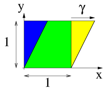
Shear of the unit square (blue) into a parallelogram (yellow)

A unit square made of a viscoelastic liquid is deformed into a parallelogram at constant shear rate, see figure on the right. The reference configuration is the unit square

${\displaystyle {\begin{pmatrix}X\\Y\end{pmatrix}}\in [0,1]^{2}}$

In the current configuration, the points of the square have the spatial coordinates

${\displaystyle {\vec {\chi }}({\vec {X}},t)={\begin{pmatrix}x\\y\end{pmatrix}}={\begin{pmatrix}X+\gamma Y\\Y\end{pmatrix}}\quad \rightarrow \quad {\dot {\vec {\chi }}}({\vec {X}},t)={\begin{pmatrix}{\dot {x}}\\{\dot {y}}\end{pmatrix}}={\begin{pmatrix}{\dot {\gamma }}Y\\0\end{pmatrix}}={\begin{pmatrix}{\dot {\gamma }}y\\0\end{pmatrix}}={\vec {v}}({\vec {x}},t)}$

from which the deformation and (spatial) speed gradient are calculated:

${\displaystyle {\begin{aligned}\mathbf {F} =&{\begin{pmatrix}1&\gamma \\0&1\end{pmatrix}}\;\rightarrow \quad {\dot {\mathbf {F} }}={\begin{pmatrix}0&{\dot {\gamma }}\\0&0\end{pmatrix}}=\operatorname {GRAD} {\dot {\vec {\chi }}}\,,\quad \mathbf {F} ^{-1}={\begin{pmatrix}1&-\gamma \\0&1\end{pmatrix}}\\\rightarrow \mathbf {l} =&\operatorname {grad} {\vec {v}}={\begin{pmatrix}0&{\dot {\gamma }}\\0&0\end{pmatrix}}={\dot {\mathbf {F} }}\cdot \mathbf {F} ^{-1}={\begin{pmatrix}0&{\dot {\gamma }}\\0&0\end{pmatrix}}\cdot {\begin{pmatrix}1&-\gamma \\0&1\end{pmatrix}}\\\rightarrow \mathbf {d} =&{\dfrac {\dot {\gamma }}{2}}{\begin{pmatrix}0&1\\1&0\end{pmatrix}}\;,\quad \mathbf {w} ={\dfrac {\dot {\gamma }}{2}}{\begin{pmatrix}0&1\\-1&0\end{pmatrix}}\,.\end{aligned}}}$

A generalization of the material law for a viscoelastic fluid (Maxwell body) with material parameters on three dimensions could look like this: ${\displaystyle \lambda {\dot {\sigma }}+\sigma =\eta \,{\dot {\varepsilon }}}$ ${\displaystyle \lambda ,\eta }$

${\displaystyle \lambda {\stackrel {\circ }{\boldsymbol {\sigma }}}+{\boldsymbol {\sigma }}=\eta \,\mathbf {d} \,.}$

Cauchy's stress tensor is deviatoric here and therefore has the form ${\displaystyle {\boldsymbol {\sigma }}}$

${\displaystyle {\boldsymbol {\sigma }}={\begin{pmatrix}\sigma &\tau \\\tau &-\sigma \end{pmatrix}}\,.}$

The Zaremba-Jaumann derivation is calculated as follows:

${\displaystyle {\stackrel {\circ }{\boldsymbol {\sigma }}}={\begin{pmatrix}{\dot {\sigma }}&{\dot {\tau }}\\{\dot {\tau }}&-{\dot {\sigma }}\end{pmatrix}}+{\frac {\dot {\gamma }}{2}}{\begin{pmatrix}\sigma &\tau \\\tau &-\sigma \end{pmatrix}}\cdot {\begin{pmatrix}0&1\\-1&0\end{pmatrix}}-{\frac {\dot {\gamma }}{2}}{\begin{pmatrix}0&1\\-1&0\end{pmatrix}}\cdot {\begin{pmatrix}\sigma &\tau \\\tau &-\sigma \end{pmatrix}}={\begin{pmatrix}{\dot {\sigma }}-{\dot {\gamma }}\tau &{\dot {\tau }}+{\dot {\gamma }}\sigma \\{\dot {\tau }}+{\dot {\gamma }}\sigma &-{\dot {\sigma }}+{\dot {\gamma }}\tau \end{pmatrix}}}$

Calculated stresses in the viscoelastic fluid at uniform shear

which leads to two differential equations for the stress components via the material law:

${\displaystyle \lambda ({\dot {\sigma }}-{\dot {\gamma }}\tau )+\sigma =0\quad {\textsf {und}}\quad \lambda ({\dot {\tau }}+{\dot {\gamma }}\sigma )+\tau ={\frac {\eta }{2}}{\dot {\gamma }}\,.}$

At constant shear rate, after eliminating the normal stress, the differential equation comes

${\displaystyle {\ddot {\tau }}+{\frac {2}{\lambda }}{\dot {\tau }}+(\lambda ^{-2}+{\dot {\gamma }}^{2})\tau ={\frac {\eta {\dot {\gamma }}}{2\lambda ^{2}}}}$

for the shear stress, which has a damped oscillation as a solution. This is a known unphysical phenomenon when using the Zaremba-Jaumann rate, see figure on the right.

Using the contravariant Oldroyd derivative yields a non-deviatoric stress tensor:

${\displaystyle {\stackrel {\nabla }{\boldsymbol {\sigma }}}={\begin{pmatrix}{\dot {\sigma }}_{xx}&{\dot {\tau }}\\{\dot {\tau }}&{\dot {\sigma }}_{yy}\end{pmatrix}}-{\begin{pmatrix}0&{\dot {\gamma }}\\0&0\end{pmatrix}}\cdot {\begin{pmatrix}\sigma _{xx}&\tau \\\tau &\sigma _{yy}\end{pmatrix}}-{\begin{pmatrix}\sigma _{xx}&\tau \\\tau &\sigma _{yy}\end{pmatrix}}\cdot {\begin{pmatrix}0&0\\{\dot {\gamma }}&0\end{pmatrix}}={\begin{pmatrix}{\dot {\sigma }}_{xx}-2{\dot {\gamma }}\tau &{\dot {\tau }}-{\dot {\gamma }}\sigma _{yy}\\{\dot {\tau }}-{\dot {\gamma }}\sigma _{yy}&{\dot {\sigma }}_{yy}\end{pmatrix}}\,.}$

The material equation gives: ${\displaystyle \lambda {\stackrel {\nabla }{\boldsymbol {\sigma }}}+{\boldsymbol {\sigma }}=\eta \,\mathbf {d} }$

${\displaystyle {\begin{pmatrix}\lambda ({\dot {\sigma }}_{xx}-2{\dot {\gamma }}\tau )+\sigma _{xx}&\lambda ({\dot {\tau }}-{\dot {\gamma }}\sigma _{yy})+\tau \\\lambda ({\dot {\tau }}-{\dot {\gamma }}\sigma _{yy})+\tau &\lambda {\dot {\sigma }}_{yy}+\sigma _{yy}\end{pmatrix}}={\frac {\eta {\dot {\gamma }}}{2}}{\begin{pmatrix}0&1\\1&0\end{pmatrix}}}$

which can be integrated in a closed manner with initially vanishing stresses and constant shear rate:

${\displaystyle {\begin{aligned}\sigma _{yy}=&0\\\tau =&{\frac {\eta {\dot {\gamma }}}{2}}(1-e^{-{\frac {t}{\lambda }}})\\\sigma _{xx}=&\eta {\dot {\gamma }}^{2}(\lambda -\lambda e^{-{\frac {t}{\lambda }}}-te^{-{\frac {t}{\lambda }}}).\end{aligned}}}$

No vibrations occur here. The figure on the right shows the stresses calculated at a shear rate of 10 / s with the Zaremba-Jaumann and the contravariant Oldroyd derivative and the material parameters given in the table. ${\displaystyle {\dot {\gamma }}=}$

parameter	Relaxation time	dynamic viscosity
Formula symbol	${\displaystyle \lambda }$	${\displaystyle \eta }$
unit	s	MPa s
Zaremba-Jaumann derivation	1.5	45.2
Contravariant Oldroyd derivative	1.5	0.2

Remarks

1. ↑ ^{a b c} The Fréchet derivative of a function according to is the restricted linear operator which - if it exists - corresponds to the Gâteaux differential in all directions, i.e. ${\displaystyle f}$ ${\displaystyle x}$ ${\displaystyle {\mathcal {A}}}$ ${\displaystyle h}$

   ${\displaystyle {\mathcal {A}}(h)=\left.{\frac {\mathrm {d} }{\mathrm {d} s}}f(x+sh)\right|_{s=0}=\lim _{s\rightarrow 0}{\frac {f(x+sh)-f(x)}{s}}\quad {\text{für alle}}\quad h}$

   applies. In it is scalar, vector or tensor valued but and similar. Then will too ${\displaystyle s\in \mathbb {R} \,,f,x\,{\textsf {und}}\,h}$ ${\displaystyle x}$ ${\displaystyle h}$

   ${\displaystyle {\mathcal {A}}={\frac {\partial f}{\partial x}}}$

   written.
2. ↑ ^{a b} Because with the vortex vector results
   ${\displaystyle {\hat {e}}\cdot \mathbf {w} \cdot {\hat {e}}={\hat {e}}\cdot ({\vec {\omega }}\times {\hat {e}})=0}$
3. ↑ Because it follows from :
   ${\displaystyle \mathbf {l} \cdot {\hat {e}}=\lambda {\hat {e}}\quad {\text{und}}\quad {\hat {e}}\cdot {\hat {e}}=1}$
   
   ${\displaystyle {\begin{aligned}\mathbf {l} \cdot {\hat {e}}-({\hat {e}}\cdot \mathbf {l} \cdot {\hat {e}}){\hat {e}}=\\=\lambda {\hat {e}}-({\hat {e}}\cdot \lambda {\hat {e}}){\hat {e}}=0\end{aligned}}}$
4. ↑ This paradox only occurs with non-material objects like the axis of rotation here or the momentary pole .
5. ↑ The symbols for the objective rates vary from source to source. The ones given here follow P. Haupt, p. 48ff. In H. Altenbach is used for and for . ${\displaystyle \mathbf {T} ^{\nabla }}$ ${\displaystyle {\stackrel {\circ }{\mathbf {T} }}}$ ${\displaystyle \mathbf {T} ^{O}}$ ${\displaystyle {\stackrel {\triangle }{\mathbf {T} }}}$
6. ↑ This derivation occurs in the Cauchy elasticity and is also named after C. Truesdell. He himself named the derivation after Cauchy and wrote in 1963 that this rate was named after him without an inventive reason ("came to be named, for no good reason, after [...] me") see C. Truesdell: Remarks on Hypo- Elasticity , Journal of Research of the National Bureau of Standards - B. Mathematics and Mathematical Physics, Vol. 67B, No. 3, July-September 1963, p. 141.

See also

• Euler equations (fluid mechanics)
• Navier-Stokes equations
• Formula collection tensor algebra
• Tensoranalysis formula collection

literature

• H. Altenbach: Continuum Mechanics . Springer, 2012, ISBN 978-3-642-24118-5 .
• P. Haupt: Continuum Mechanics and Theory of Materials . Springer, 2000, ISBN 3-540-66114-X .

Individual evidence

1. ↑ Altenbach (2012), pp. 109 and 32.
2. ↑ after James G. Oldroyd (1921 - 1982), James G. Oldroyd in engl. Wikipedia (engl.)
3. ↑ P. Haupt (2000), pp. 302ff