Potential flow

The flow of a fluid (liquid or gas) is a potential flow if the vector field of the velocities is mathematically such that it has a potential . Such a potential is in a homogeneous available fluid when the flow irrotational (d. H. Vortex or vortizitätsfrei ) and no viscous forces ( frictional forces ) occur or are negligibly small. Every flow of a homogeneous, frictionless fluid that begins at rest has such a potential.

A potential flow is the rotation-free special case of the flow of a homogeneous, frictionless fluid, which is described by Euler's equations ; these also apply to currents with rotation (eddy currents). If, however, the toughness must be taken into account in shear movements , such as B. in boundary layers or in the center of a vortex, the Navier-Stokes equations must be used.

Potential flows can be used as a very good approximation of laminar flows at low Reynolds numbers if the fluid dynamic boundary layer at the edges of the flow does not play an essential role. In the steady potential flow of incompressible fluids, the Bernoullian pressure equation applies globally, which describes technical pipe flows well. Because they are easy to calculate, potential flows are also used as an initial approximation in the iterative calculation of the Navier-Stokes equations in numerical fluid mechanics .

definition

A potential flow is a flow that has a velocity field that depends on the location and the time t and is calculated from the gradient "grad" of a velocity potential : ${\displaystyle {\vec {v}}({\vec {x}},t)}$ ${\displaystyle {\vec {x}}}$ ${\displaystyle \phi ({\vec {x}},t)}$

${\displaystyle {\vec {v}}=\operatorname {grad} (\phi )\quad \Leftrightarrow \quad v_{i}={\frac {\partial \phi }{\partial x_{i}}}\,,\;i=1,2,3\,.}$

That is why such flows are called potential flows. The left vector equation is the coordinate-free version, while the right equations are in Cartesian coordinates . ${\displaystyle x_{1,2,3}}$

Every gradient field is rotation-free , which is why potential flows are always rotation-free. Conversely, according to the Poincaré lemma , a velocity potential always exists when the flow is rotation-free.

Areas of application and limitations

Potential flows do not contain all the characteristics of real flows. The incompressible potential flow makes a number of false predictions, such as the d'Alembert paradox , according to which no force is exerted on a body in the direction of the flow. All phenomena that involve a hydrodynamic boundary layer or turbulent flow along with the dissipation of energy, such as B. flow breaks cannot be mapped with potential flows.

Nevertheless, the understanding of potential flows is helpful in many areas of fluid mechanics. For geometries that are not too complicated, analytical solutions for the flow around them can be calculated and the buoyancy force provided by the flow can also be specified. In this way, a deeper understanding of the flow is achieved.

Potential currents have many applications in the design of aircraft. As mentioned at the beginning, potential flows can be used as a very good approximation of laminar flows at low Reynolds numbers if the hydrodynamic boundary layer at the edges of the flow does not play an essential role. A technique in computational fluid mechanics couples a viscous boundary layer flow to a potential flow outside the boundary layer. In a potential flow, any streamline can be replaced by a wall without changing the flow, a technique used in aircraft design.

Determining equations for the flow

Not every velocity potential represents a physically plausible flow. In order for the velocity potential to be in accordance with the laws of physics under the assumptions made, it must obey the momentum balance in the form of Euler's equations and meet the mass balance .

Balance equations

The balance equation for the momentum, in the form of Euler's equations, is

${\displaystyle {\frac {\partial {\vec {v}}}{\partial t}}+\operatorname {grad} ({\vec {v}})\cdot {\vec {v}}+{\frac {1}{\rho }}\operatorname {grad} (p)={\vec {k}}}$

and the mass balance

${\displaystyle {\dot {\rho }}+\rho \operatorname {div} ({\vec {v}})=0\,.}$

Here, ρ is the density and the point on top is the substantial time derivative , “div” is the divergence of a vector field , p is the pressure and an acceleration field (e.g. acceleration due to gravity). This system of four equations with five unknowns (three speeds, pressure and density) is closed by an equation of state that represents pressure as a function of density. ${\displaystyle {\vec {k}}}$

Inserting the potential into Euler's equations yields with the Graßmann expansion:

${\displaystyle {\begin{aligned}{\frac {\partial {\vec {v}}}{\partial t}}+\operatorname {grad} ({\vec {v}})\cdot {\vec {v}}+{\frac {1}{\rho }}\operatorname {grad} (p)&={\vec {k}}\\{\frac {\partial {\vec {v}}}{\partial t}}+{\frac {1}{2}}\operatorname {grad} ({\vec {v}}\cdot {\vec {v}})-{\vec {v}}\times \operatorname {rot} ({\vec {v}})+{\frac {1}{\rho }}\operatorname {grad} (p)&={\vec {k}}\\\Rightarrow \operatorname {grad} \left({\frac {\partial \phi }{\partial t}}+{\frac {1}{2}}\operatorname {grad} (\phi )^{2}\right)+{\frac {1}{\rho }}\operatorname {grad} (p)&={\vec {k}}\,,\end{aligned}}}$

because the rotation of a gradient field disappears. The mass balance is formed with the velocity potential and the Laplace operator to: ${\displaystyle \Delta =\operatorname {div\circ grad} }$

${\displaystyle {\dot {\rho }}+\rho \operatorname {div(grad} (\phi ))={\dot {\rho }}+\rho \Delta \phi =0\,.}$

Now it is a system of four equations with three unknowns (potential, pressure and density), which can only be solved if the difference fulfills the integrability condition. This is the case in barotropic fluids in a conservative gravitational field. ${\displaystyle {\vec {f}}:={\vec {k}}-{\tfrac {1}{\rho }}\operatorname {grad} (p)}$ ${\displaystyle \operatorname {rot} ({\vec {f}})={\vec {0}}}$

Barotropic fluid in a conservative gravitational field

In a barotropic fluid, the density is only a function of the pressure. Then the integration of the Euler equations can take place in advance, which simplifies the calculation considerably.

A function P with the property

${\displaystyle P:=\int {\frac {\mathrm {d} p}{\rho (p)}}\quad \Leftrightarrow \quad \mathrm {d} P={\frac {\mathrm {d} p}{\rho }}\quad \Leftrightarrow \quad \operatorname {grad} P={\frac {1}{\rho }}\operatorname {grad} p\,.}$

Are defined. In an incompressible fluid the density is constant and P = p / ρ. Inserting the function P into the Euler equation allows to extract the gradient operator:

${\displaystyle \operatorname {grad} \left({\frac {\partial \phi }{\partial t}}+{\frac {1}{2}}\operatorname {grad} (\phi )^{2}\right)+{\frac {1}{\rho }}\operatorname {grad} (p)=\operatorname {grad} \left({\frac {\partial \phi }{\partial t}}+{\frac {1}{2}}\operatorname {grad} (\phi )^{2}+P\right)={\vec {k}}\,.}$

So that this equation can be fulfilled, the acceleration field must correspond to the integrability condition . Then according to the Poincaré lemma there is a potential V with the property and the above equation leads to a gradient field ${\displaystyle {\vec {k}}}$ ${\displaystyle \operatorname {rot} {\vec {k}}={\vec {0}}}$ ${\displaystyle {\vec {k}}=-\operatorname {grad} V}$

${\displaystyle \operatorname {grad} \left({\frac {\partial \phi }{\partial t}}+{\frac {1}{2}}\operatorname {grad} (\phi )^{2}+P+V\right)={\vec {0}}\,,}$

that disappears everywhere, which is why the term in the big brackets is location-independent:

${\displaystyle {\frac {\partial \phi }{\partial t}}+{\frac {1}{2}}\operatorname {grad} (\phi )^{2}+P+V=C\,.}$

The integration constant C could still depend on the time, but this time dependency can be added to the potential without its physical meaning changing. ${\displaystyle \phi }$ ${\displaystyle \operatorname {grad} (\phi )={\vec {v}}}$

Now it is a closed system of three equations (including ρ = ρ (p) and the mass balance) with three unknowns potential, density and pressure.

Stationary flow

In a steady potential flow without an acceleration field, the following applies:

${\displaystyle \left(1-M_{x}^{2}\right){\frac {\partial ^{2}\phi }{\partial x^{2}}}+\left(1-M_{y}^{2}\right){\frac {\partial ^{2}\phi }{\partial y^{2}}}+\left(1-M_{z}^{2}\right){\frac {\partial ^{2}\phi }{\partial z^{2}}}-2M_{x}M_{y}{\frac {\partial ^{2}\phi }{\partial x\,\partial y}}-2M_{y}M_{z}{\frac {\partial ^{2}\phi }{\partial y\,\partial z}}-2M_{z}M_{x}{\frac {\partial ^{2}\phi }{\partial z\,\partial x}}=0,}$

with the Mach numbers

${\displaystyle M_{x}={\frac {1}{c}}{\frac {\partial \phi }{\partial x}},\qquad M_{y}={\frac {1}{c}}{\frac {\partial \phi }{\partial y}},\qquad {\text{und}}\qquad M_{z}={\frac {1}{c}}{\frac {\partial \phi }{\partial z}},}$

and the local speed of sound c . The flow velocity results from the gradient of the velocity potential. These equations are applicable to sub- , trans- and supersonic flow as long as they are free of rotation. ${\displaystyle {\vec {v}}=\operatorname {grad} (\phi )}$

proof

In a steady flow without an acceleration field, the Euler equation and the mass balance reads: Here the speed of sound occurs, which is the root of the derivation of the pressure with respect to the density with constant entropy S. Scalar multiplication of the Euler equation with the speed and onset of the mass balance yields: Division by yields with the speed potential and the Mach number : ${\displaystyle {\begin{aligned}\operatorname {grad} ({\vec {v}})\cdot {\vec {v}}&=-{\frac {1}{\rho }}\operatorname {grad} (p)=-{\frac {c^{2}}{\rho }}\operatorname {grad} (\rho )\\\operatorname {div} (\rho {\vec {v}})&=\operatorname {grad} (\rho )\cdot {\vec {v}}+\rho \operatorname {div} ({\vec {v}})=0\end{aligned}}}$ ${\displaystyle c={\sqrt {\left.{\frac {\partial p}{\partial \rho }}\right|_{S}}}}$ ${\displaystyle {\vec {v}}\cdot \operatorname {grad} ({\vec {v}})\cdot {\vec {v}}=-{\frac {c^{2}}{\rho }}\operatorname {grad} (\rho )\cdot {\vec {v}}={\frac {c^{2}}{\rho }}\rho \operatorname {div} ({\vec {v}})=c^{2}\operatorname {div} ({\vec {v}})\,.}$ ${\displaystyle c^{2}}$ ${\displaystyle {\vec {M}}:={\vec {v}}/c=\operatorname {grad} (\phi )/c}$ ${\displaystyle {\vec {M}}\cdot \operatorname {grad(grad} (\phi ))\cdot {\vec {M}}=\operatorname {div(grad} (\phi ))=\Delta \phi \quad \Leftrightarrow \quad \sum _{i=1}^{3}{\frac {\partial ^{2}\phi }{\partial x_{i}^{2}}}-\sum _{i,j=1}^{3}M_{i}M_{j}{\frac {\partial ^{2}\phi }{\partial x_{i}\partial x_{j}}}=0\,.}$

In the sub- or supersonic range (but not in the transonic), a further assumption can be made with small angles of incidence of slender bodies: The velocity potential is divided into a parallel flow and a small interference field : In this case, the linearized potential equation - an approximation of the complete equation - to be used: ${\displaystyle v_{\infty }x}$ ${\displaystyle \varphi }$ ${\displaystyle \phi =v_{\infty }x+\varphi \,.}$

${\displaystyle (1-M_{x}^{2}){\frac {\partial ^{2}\varphi }{\partial x^{2}}}+{\frac {\partial ^{2}\varphi }{\partial y^{2}}}+{\frac {\partial ^{2}\varphi }{\partial z^{2}}}=0\,.}$

Sound waves

Sound waves with low amplitudes can be approximated with the following potential flow model:

${\displaystyle {\frac {\partial ^{2}\phi }{\partial t^{2}}}={\bar {c}}^{2}\Delta \phi \,.}$

This is the mean speed of sound in the homogeneous fluid. This equation is a wave equation that applies to the velocity potential Φ and also to the pressure and density. ${\displaystyle {\bar {c}}}$

boundary conditions

The Dirichlet boundary conditions specify the value of the velocity potential on a surface, from which the tangential velocity of the fluid on the surface results. With Neumann boundary conditions , the derivatives of the potential perpendicular to surfaces are determined, which here corresponds to the specification of velocity components perpendicular to the surface. Otherwise, what was said about the boundary conditions for Euler's equations applies.

Potential flow of an incompressible fluid

The assumption of incompressibility is often a sensible approximation for liquids at moderate pressures and for gas flows well below the speed of sound. In this case, the equations for determining the speed and pressure are decoupled: The potential is determined from the Laplace equation with the boundary conditions and the pressure is determined from the Euler equations, which are reduced to Bernoulli's pressure equation.

Determining equations

In the case of incompressibility, the velocity field is free of divergence

${\displaystyle \operatorname {div} {\vec {v}}=\operatorname {div(grad} (\phi ))=\Delta \phi =0\,,}$

hence the potential satisfies the Laplace equation . Due to the mass balance , the density is constant over time and space. At constant density, the function P introduced for barotropic fluids is simplified to P = p / ρ. Multiplying the Euler equations by the density then yields: ${\displaystyle {\dot {\rho }}+\rho \Delta \phi ={\dot {\rho }}=0}$

${\displaystyle \rho {\frac {\partial \phi }{\partial t}}+{\frac {\rho }{2}}\operatorname {grad} (\phi )^{2}+p+\rho V=E\,.}$

In a steady flow, the first term does not apply and Bernoulli's pressure equation remains , which applies here to the entire flow area. The constant energy E is the sum of the kinetic, internal (pressure p) and external energy (gravitational field ρV) of a fluid particle and this total energy is the same for all particles in the steady flow.

Analog of thermal conduction

→ Main article : Thermal conduction

Comparison of the flow calculated via heat conduction (colored and black) with the analytical streamlines (white)

The square of the amount of heat flow corresponds to the pressure distribution

A potential flow can be calculated with finite element programs, in which the heat conduction equation is implemented, which is the case in many common programs. The stationary heat conduction in a homogeneous solid body without internal heat sources obeys the Laplace equation

${\displaystyle \Delta T=0\,,}$

which is why the temperature T there is subject to the same equation as the velocity potential Φ in an incompressible fluid. If the temperature in a solid is understood as a velocity potential, then the temperature gradient, to which the heat flow is proportional, corresponds to the flow velocity. The Dirichlet boundary conditions determine the temperatures on surfaces, whereby the temperature gradient and thus the tangential flow velocity in the surface can be specified. Neumann boundary conditions determine the heat flow density, which sets the normal velocity to the wall in the potential flow.

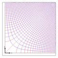
The picture above shows a section of the temperature distribution from a heat conduction calculation using the finite element method in a square disc with a profile cut out in the center, which is treated in the example below. The temperature is color-coded from red to blue (red high, blue low) and the black lines running from top to bottom are its contour lines. The short, black lines, oriented from left to right, represent heat flows. In order to keep edge effects low, the disk is ten times as large as the profile, because the analytically calculated, white drawn flow lines in the example below apply to a flow throughout the entire, wall-free level. No boundary conditions have been defined at the borders of the pane (outside the image) above and below or on the profile. The heat flux density of one was specified on the left edge and the heat flow density of minus one on the right edge and the temperature zero in the middle. With a constant temperature at the right limit, a vertical discharge would have been determined. The contour lines of the temperature correspond to the contour lines of the velocity potential and, in accordance with the theory, are apparently perpendicular to the white streamlines and the heat flows are compatible with the streamlines.

The lower picture shows the square of the amount of heat flow (red large, blue small), of which according to the Bernoulli equation without gravitational acceleration

${\displaystyle p=E-{\frac {\rho }{2}}\operatorname {grad} (\phi )^{2}}$

the pressure is a linear function. Because of the negative sign, there is a high pressure in the blue areas and a lower pressure in the red.

Plane potential flow

If the flow takes place in the plane, then the properties of complex functions can be exploited. A complex speed potential is defined, the real part of which is the real speed potential and the imaginary part of which is the current function . Both functions describe the same flow. Therefore the statements derived from the flow function apply: The contour lines of the flow function are flow lines between which the volume flow is the same everywhere. Complex velocity potentials can be assembled from simpler ones and transformed so that complicated flows can be investigated with simple means. In particular, the force exerted on the body by the flow can also be precisely calculated.

Complex speed potential

The plane is understood as a complex number plane in which the value of the potential is represented as the real part of a holomorphic function f:

${\displaystyle f(z)=\phi (x,y)+\mathrm {i} \,\psi (x,y)\quad {\text{mit}}\quad z=x+\mathrm {i} \,y\in \mathbb {C} \,.}$

The set contains all complex numbers and i is the imaginary unit . The function f is the complex speed potential, from which the speed is derived via the derivatives ${\displaystyle \mathbb {C} }$

${\displaystyle v_{x}={\frac {\partial \phi }{\partial x}}\;,\quad v_{y}={\frac {\partial \phi }{\partial y}}\quad {\text{oder}}\quad w:=v_{x}-\mathrm {i} \,v_{y}={\frac {\mathrm {d} f}{\mathrm {d} z}}}$

results. Here w is the complex velocity . The imaginary part of the potential is the current function , the contour lines of which are streamlines . Because the function f is holomorphic, the Cauchy-Riemann differential equations apply

${\displaystyle {\frac {\partial \phi }{\partial x}}={\frac {\partial \psi }{\partial y}}\quad {\text{und}}\quad {\frac {\partial \phi }{\partial y}}=-{\frac {\partial \psi }{\partial x}}\,.}$

which is why the gradients of the real velocity potential and the current function are mutually perpendicular:

${\displaystyle \operatorname {grad} (\phi )\cdot \operatorname {grad} (\psi )=0\,.}$

The gradients are again orthogonal to the contour lines, so that these also intersect at right angles. Further differentiation revealed

${\displaystyle {\begin{aligned}{\frac {\partial ^{2}\phi }{\partial x^{2}}}&={\frac {\partial ^{2}\psi }{\partial y\partial x}}=-{\frac {\partial ^{2}\phi }{\partial y^{2}}}\quad \Rightarrow \quad \Delta \phi =0\\{\frac {\partial ^{2}\psi }{\partial y^{2}}}&={\frac {\partial ^{2}\phi }{\partial x\partial y}}=-{\frac {\partial ^{2}\psi }{\partial x^{2}}}\quad \Rightarrow \quad \Delta \psi =0\,,\end{aligned}}}$

therefore both the real and the imaginary part of the complex velocity potential satisfy the Laplace equation in the plane. The upper equation defines the freedom of divergence and the lower one the freedom of rotation of the flow.

The potential is calculated from the boundary conditions, from which the velocity field is calculated via the derivatives, and the pressure is determined from Bernoulli's pressure equation.

Approximate arithmetic solution

The Laplace operator has the difference quotient in the plane in a regular network with mesh size ${\displaystyle \triangle x=\triangle y=h}$

${\displaystyle {\begin{aligned}\Delta \psi =&{\frac {\triangle ^{2}\psi }{\triangle x^{2}}}+{\frac {\triangle ^{2}\psi }{\triangle y^{2}}}\\=&{\frac {\psi (x+h,y)+\psi (x-h,y)-2\psi (x,y)}{h^{2}}}+{\frac {\psi (x,y+h)+\psi (x,y-h)-2\psi (x,y)}{h^{2}}}{\stackrel {\displaystyle !}{=}}0\\\rightarrow \psi (x,y)=&{\frac {\psi (x+h,y)+\psi (x-h,y)+\psi (x,y+h)+\psi (x,y-h)}{4}}\end{aligned}}}$

The differences were also written to avoid confusion with the Laplace operator. The formula allows a simple solution of the Laplace equation: A net with square meshes with edge length h is placed in the flow area . The value of the current function at the node with coordinates ( x , y ) is then the mean value of the neighboring node values ​​in the x and y directions. In the case of a flow-through channel, the flow function is set to zero on one edge and the value that corresponds to the required volume flow is set on the opposite edge. For the node values ​​in the flow area, estimated values ​​are first used and then iteratively adjusted using the above equation until a satisfactory accuracy is achieved. ${\displaystyle \triangle }$

Drawing determination of potential flows

→ Main article : flow network

In six steps, manually created drawing of a potential flow around an open helicopter using Xfig

Potential flows can also be sketched by hand, which is used in geotechnics and hydromechanics . The properties of planar potential flows listed above provide information on this:

• Impermeable edges or free surfaces are streamlines,
• Streamlines must not intersect,
• Potential lines must not intersect,
• Potential lines and streamlines intersect at right angles and
• the network of potential and current lines can be designed so that it consists of approximately square meshes.

At the beginning the edges of the flow area are drawn (step 1 in the picture) and the direction of the flow at the inlet and outlet is determined (2). Then (3) a few parallel streamlines are laid between the edges of the flow area at equal intervals, taking into account that the edges are also streamlines. The potential lines are drawn in such a way (4) that they cross these streamlines at right angles and square meshes are created. By entering further current and potential lines (5,6), the network is compressed to the desired extent.

Construction of speed potentials

Because Laplace's equation is linear, the flow that results from the sum of two velocity potentials is again a potential flow. Complex flows can be composed of simple flows by superposition, some of which - see the images below - are given:

1. A parallel flow with constant complex speed results from . ${\displaystyle w=v_{x}-\mathrm {i} \,v_{y}}$ ${\displaystyle f(z)=wz}$
2. A stagnation point flow with a stagnation point at the origin results with ${\displaystyle f(z)=z^{n}\,,\;n=2,3,4,\dots }$
3. A multipole flow at the origin has the potential ${\displaystyle f(z)=z^{-n}\,,\;n=1,2,3,4,\dots }$
4. Sources have a potential of the form The location of the source is , its strength is Q and ln is the natural logarithm . At the point there is a singularity in which the Laplace equation is violated. Sinks are sources of negative strength. ${\displaystyle f(z)={\frac {Q}{2\pi }}\ln(z-z_{0})\,.}$ ${\displaystyle z_{0}}$ ${\displaystyle z=z_{0}}$
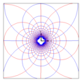
5. The potential vortex - see below - results from interchanging the real and imaginary parts in a source flow, which is done by multiplying the potential by -i: ${\displaystyle f(z)=-\mathrm {i} \,{\frac {\Gamma }{2\pi }}\ln(z-z_{0})\,.}$
6. Vortices result from the superposition of sources / sinks and potential vortices: ${\displaystyle f(z)={\frac {Q-\mathrm {i} \,\Gamma }{2\pi }}\ln(z-z_{0})\,.}$

• 

  Parallel flow

• 

  Stagnation point flow

• 

  Multipole flow

• 

  Source / sink

• 

  whirl

• 

  swirl

In the pictures above, the contour lines of the real potential are drawn in red and those of the current function in blue. The distance between the red lines gives an impression of the flow speed, whereby the speed is high in areas with small distances. The blue lines are streamlines. The functions, the contour lines of which run radially at the sources / sinks, eddies or vortices, make a jump somewhere, which is a consequence of the non-differentiability of the logarithmic function.

With the method of image charges , the flow can be deflected by cleverly introducing imaginary sources and sinks outside the area through which the flow passes, so that it fulfills specified boundary conditions.

With conformal images , flow fields around simple base bodies can be transferred to complex geometries. The transfer takes place with a second, complex function w according to which conforms to Riemann's mapping theorem . The Kutta-Schukowski transformation transfers the flow around a circular cylinder to a wing profile, see the example below. With the Schwarz-Christoffel transformation , the parallel flow in the upper half-plane can be transferred to any simply contiguous areas bordered by straight lines (and also the interior of polygons ). ${\displaystyle \Pi (z)=w(f(z))\,,}$

Effects of forces on bodies in a flow

The d'Alembert paradox states that no force acts in the direction of the flow on any body of any shape. In a complex differentiable velocity field, the flow does not exert any force perpendicular to the direction of flow on bodies around which it flows, which is a consequence of Cauchy's integral theorem . If the velocity potential cannot be complexly differentiated anywhere within the contour of a body, then the circulation of the velocity along the contour can be unequal to zero and, according to Kutta-Joukowski's theorem, the body experiences a buoyancy force proportional to this circulation. With the formula discovered in 1902, the first lift-generating wing profiles could be developed.

An important variable when calculating the force effect on bodies in flow is the circulation Γ of the speed along a path W, which is calculated using a curve integral :

${\displaystyle \Gamma :=\oint _{W}(v_{x}\mathrm {d} x+v_{y}\,\mathrm {d} y)\,.}$

If the curve is a contour with a flow around it, then the circulation can be calculated with the complex velocity:

${\displaystyle \Gamma =\oint _{W}w(z)\,\mathrm {d} z\quad (\in \mathbb {R} )\,.}$

The integral set of Cauchy states that the line integral of a complex function between two points is independent of the path when the function holomorphic thus is complex differentiable. The curve integral accordingly disappears along a closed contour if the function is holomorphic in the area enclosed by the contour. The circulation can only differ from zero if the velocity field cannot be complexly differentiated somewhere within the contour.

The complex force ( acting in the positive y-direction), which acts on a body around which a planar potential flow flows, whose constant cross-section is the planar contour W and whose extension perpendicular to the cross-section is L, is calculated using the first Blasius formula ${\displaystyle F=F_{x}-\mathrm {i} F_{y}}$ ${\displaystyle F_{y}}$

${\displaystyle F=\mathrm {i} L{\frac {\rho }{2}}\oint _{W}w^{2}(z)\,\mathrm {d} z}$

with the curve integral of the speed square along the contour. The set of Kutta Joukowski states that the force that acts on the immersed body is proportional to its circulation:

${\displaystyle F=\mathrm {i} L\rho \Gamma w_{\infty }=L\rho \Gamma e^{\mathrm {i} {\frac {\pi }{2}}}w_{\infty }\,.}$

Because the force is always perpendicular to the flow velocity at infinity, the force is also called the buoyancy force. In eddy-free currents, the circulation disappears, so that an eddy-free potential current does not exert any force on bodies around which it flows. ${\displaystyle w_{\infty }}$

Potential vortex

The potential vortex or "free vortex" is a real (rotation-free) potential flow that nevertheless circles, i. H. has a circulation in a topologically twofold connected area (such as the air space in a hall with a central column) . A special potential vortex can be observed on a free water surface when the pressure in the center becomes so low that the surface sinks noticeably and forms a vortex funnel ( vortex ). If the funnel extends indefinitely into the depth, there is potential flow in the entire liquid area, but not in the air-filled core.

In the case of a free vortex, all fluid particles move on concentric circular paths with amounts of velocity that (except in the core area) correspond to the law of distance with constant  and axis spacing  : ${\displaystyle v(r)}$ ${\displaystyle c}$ ${\displaystyle r}$

${\displaystyle v(r)={\frac {c}{r}}}$

It is a reciprocal proportionality , i. H. the further away from the axis the particles are, the slower they move, and the innermost particles move the fastest. This results in a completely different speed and pressure distribution than in the quasi-rigid vortex, which has no potential and whose speed is proportional to the axis distance: ${\displaystyle v=\omega \cdot r.}$

In real fluids, free eddies are only approximately formed as potential flows, since viscous forces in their middle lead to a quasi-rigid rotation and the velocity field here has vorticity.

According to Bestehorn, the potential vortex is actually a point vortex: The complex potential of the vortex is as indicated above: ${\displaystyle z-z_{0}=re^{\mathrm {i} \,\varphi }}$

${\displaystyle f(z)=-\mathrm {i} \,{\frac {\Gamma }{2\pi }}\ln(z-z_{0})=-\mathrm {i} \,{\frac {\Gamma }{2\pi }}\ln \left(re^{\mathrm {i} \,\varphi }\right)={\frac {\Gamma }{2\pi }}\varphi -\mathrm {i} \,{\frac {\Gamma }{2\pi }}\ln(r)\,.}$

On the negative real axis at the complex natural logarithm is not differentiable, which is why the potential is not at all. However, the current function that fully describes the vortex can be used. The vortex strength is ${\displaystyle \varphi =\pm n\pi \,,\;n=1,3,5,\ldots }$ ${\displaystyle \psi =-{\frac {\Gamma }{2\pi }}\ln(r)\,,}$

${\displaystyle \omega =-{\frac {1}{2}}\Delta \psi ={\frac {1}{2}}\Gamma \delta (z-z_{0})\,,}$

with the Dirac delta "δ", which is why the potential vortex is an infinitely strong point vortex at the point , see Hamel-Oseenscher vortex . ${\displaystyle z=z_{0}}$

example

Plane potential flow around a cylinder and a wing profile

The complex speed potential

${\displaystyle f(z)=z+{\frac {1}{z}}=x+\mathrm {i} \,y+{\frac {1}{x+\mathrm {i} \,y}}=\underbrace {x+{\frac {x}{x^{2}+y^{2}}}} _{=\phi }+\mathrm {i} \underbrace {\left(y-{\frac {y}{x^{2}+y^{2}}}\right)} _{=\psi }}$

describes the flow around a cylinder, because its circumference at is a streamline with ψ = 0, see the upper part of the figure. The streamlines are contour lines of the stream function ψ and have the equation ${\displaystyle x^{2}+y^{2}=1}$

${\displaystyle y-{\frac {y}{x^{2}+y^{2}}}=\psi \quad \Rightarrow \quad x=\pm {\sqrt {{\frac {y}{y-\psi }}-y^{2}}}}$

and are drawn in white in the picture at a distance of Δψ = 0.3. The streamline with ψ = 0 is drawn in red. The speed is obtained by deriving the speed potential:

${\displaystyle v_{x}-\mathrm {i} \,v_{y}={\frac {\mathrm {d} f}{\mathrm {d} z}}=1-{\frac {1}{z^{2}}}\quad \Rightarrow \quad v^{2}=\left(1-{\frac {1}{z^{2}}}\right){\overline {\left(1-{\frac {1}{z^{2}}}\right)}}=1+{\frac {2(y^{2}-x^{2})+1}{(x^{2}+y^{2})^{2}}}\,.}$

In the absence of a gravitational field, the Bernoulli equation gives the pressure:

${\displaystyle {\frac {\rho }{2}}v^{2}+p=E\quad \Rightarrow \quad p=E-{\frac {\rho }{2}}\left(1+{\frac {2(y^{2}-x^{2})+1}{(x^{2}+y^{2})^{2}}}\right)}$

With the compliant mapping

${\displaystyle w(z)=z+z_{0}+{\frac {R^{2}}{z+z_{0}}}\quad {\text{mit}}\quad R=\Re (z_{0})+{\sqrt {1-\Im (z_{0})^{2}}}}$

the cylinder is transformed to a contour that resembles a wing profile, see the lower part of the picture where and is. The functions and extract the real or imaginary part of their complex argument. The amount of controls the bulge, while the phase affects the curvature of the profile. ${\displaystyle z_{0}=0{,}15\,e^{\mathrm {i} {\frac {5}{6}}\pi }}$ ${\displaystyle R=0{,}8672}$ ${\displaystyle \Re }$ ${\displaystyle \Im }$ ${\displaystyle z_{0}}$

The flow is transformed like the contour, so that the streamlines are in the w-plane with

${\displaystyle w(z)=z+z_{0}+{\frac {R^{2}}{z+z_{0}}}\quad {\text{und}}\quad z=\pm {\sqrt {{\frac {y}{y-\psi }}-y^{2}}}+\mathrm {i} \,y}$

surrender. They are drawn in white in the lower part of the picture. The streamlines of this profile were compared above, in the section #Analogon of thermal conduction , with the results from a thermal conduction analysis .

Footnotes

1. ↑ ${\displaystyle \operatorname {grad} ({\vec {f}})\cdot {\vec {f}}={\frac {1}{2}}\operatorname {grad} ({\vec {f}}\cdot {\vec {f}})-{\vec {f}}\times \operatorname {rot} ({\vec {f}})}$

Individual evidence

1. ^ R. Greve: Continuum Mechanics . 2003, p. 147 .
2. ^ ^{A b c} John D. Anderson : Modern compressible flow. With historical perspective . McGraw-Hill, New York NY 2002, ISBN 0-07-242443-5 , pp. 358-359 .
3. ↑ Horace Lamb : Hydrodynamics. 6th edition. Cambridge University Press, Cambridge 1993, ISBN 0-521-05515-6 , pp. 492-495.
4. ↑ ^{a b} A. Malcherek: Hydromechanics for civil engineers. (pdf) Universität der Bundeswehr München, p. 48ff , accessed on October 9, 2016 (German). 
5. ^ M. Bestehorn: hydrodynamics and structure formation. 2006, p. 95.
6. ^ M. Bestehorn: hydrodynamics and structure formation. 2006, p. 87.
7. ^ M. Bestehorn: hydrodynamics and structure formation. 2006, p. 91 ff.

literature

• Michael Bestehorn: hydrodynamics and structure formation . Springer, Berlin et al. 2006, ISBN 3-540-33796-2 .
• Ralf Greve: Continuum Mechanics. A basic course for engineers and physicists . Springer, Berlin et al. 2003, ISBN 3-540-00760-1 .
• Hans J. Lugt: Eddy currents in nature and technology. G. Braun, Karlsruhe 1979, ISBN 3-7650-2028-1 .
• Herbert Oertel (ed.): Prandtl guide through fluid mechanics. Fundamentals and phenomena. 11th, revised and expanded edition. Vieweg, Braunschweig et al. 2002, ISBN 3-528-48209-5 .
• Heinz Schade, Ewald Kunz: Fluid Mechanics. 2nd, revised and improved edition. de Gruyter, Berlin et al. 1989, ISBN 3-11-011873-4 .
• Jürgen Zierep: Basics of fluid mechanics. 4th, revised edition. G. Braun, Karlsruhe 1990, ISBN 3-7650-2039-7 .

Web links

• mathfaculty.fullerton.edu with many examples of conformal mapping , accessed on August 16, 2015.