Euler equations (fluid mechanics)

Current around a wing. This incompressible flow satisfies the Euler equations.

The Euler equations (or Euler's equations ) of fluid mechanics are a mathematical model developed by Leonhard Euler to describe the flow of frictionless elastic fluids . In the narrower sense, Euler equations mean the momentum equation for frictionless flows. This is sometimes referred to as Euler's equation . In a broader sense, this is expanded to include the continuity equation and the energy equation and then forms a system of non-linear partial differential equations of the first order.

The corresponding momentum equations are formulated in Eulerian perspective and are:

${\displaystyle {\frac {\partial {\vec {v}}}{\partial t}}+({\vec {v}}\cdot \nabla ){\vec {v}}+{\frac {1}{\rho }}\operatorname {grad} (p)={\vec {k}}\quad \iff \quad {\frac {\partial v_{i}}{\partial t}}+\sum _{j=1}^{3}{\frac {\partial v_{i}}{\partial x_{j}}}v_{j}+{\frac {1}{\rho }}{\frac {\partial p}{\partial x_{i}}}=k_{i}\;,\quad i=1,2,3\,.}$

The vector is the velocity field in the fluid with components in the direction of the Cartesian coordinates , the density , the pressure and an external volume-distributed acceleration (e.g. acceleration due to gravity). The vector gradient corresponds to the product of the velocity and speed: . All variables in the Euler equations are generally dependent on both location and time. The left vector equation is the coordinate-free version that applies in any coordinate system, and the right component equations result in the special case of the Cartesian coordinate system. ${\displaystyle {\vec {v}}}$ ${\displaystyle v_{1,2,3}}$ ${\displaystyle x_{1,2,3}}$ ${\displaystyle \rho }$ ${\displaystyle p}$ ${\displaystyle {\vec {k}}}$ ${\displaystyle ({\vec {v}}\cdot \nabla ){\vec {v}}}$ ${\displaystyle ({\vec {v}}\cdot \nabla ){\vec {v}}=\operatorname {grad} ({\vec {v}})\cdot {\vec {v}}}$

The Navier-Stokes equations contain these equations as the special case in which the internal friction ( viscosity ) and the heat conduction of the fluid are neglected. The Euler equations are used for laminar flows , as they can be assumed to a good approximation in technical pipe flows or in aircraft development. In the case of incompressibility , the Bernoulli equation can be derived from the Euler equations , and with an additional eddy-free flow, potential flows result .

Derivation

The Euler equations can be derived in different ways: A common approach applies Reynolds' transport theorem to Newton's second axiom . The transport theorem describes the change over time of a physical quantity in a moving control volume.

Another approach is based on the Boltzmann equation : The collision operator is multiplied by three possible terms, the so-called collision invariants. After integration over the particle speed, the continuity equation, momentum equation and energy balance arise. Finally, a scaling for large time and space dimensions is carried out ( hydrodynamic limits ), and the result is the extended Euler equations.

formulation

Momentum equation

The essential part of the Euler equations is the first Cauchy-Euler law of motion , which corresponds to the momentum theorem :

${\displaystyle \rho \left[{\frac {\partial }{\partial t}}{\vec {v}}+\operatorname {grad} ({\vec {v}})\cdot {\vec {v}}\right]=\rho \,{\vec {k}}+\operatorname {div} ({\boldsymbol {\sigma }})\,.}$

On the left side of the equation, in square brackets, is the substantial acceleration , consisting of the local and convective acceleration:

${\displaystyle {\frac {\mathrm {D} {\vec {v}}}{\mathrm {D} t}}={\frac {\partial {\vec {v}}}{\partial t}}+\operatorname {grad} ({\vec {v}})\cdot {\vec {v}}\;.}$

In addition to the variables described above, the Cauchy stress tensor and the divergence operator appear. Internal friction, which would show up in viscosity and thus in shear stresses, is neglected in elastic fluids, which is why the stress tensor there has a diagonal shape. Furthermore, every fluid is also isotropic . If a fluid is now mentally cut into two parts, then cutting stresses develop on the cut surfaces that are perpendicular to the cut surface, because the pressure in an elastic fluid always acts perpendicularly on the delimiting surfaces. In an isotropic liquid, the normal stress must for all orientations of the cut surface be the same so the stress tensor therefore a multiple of Einheitstensors is . A stress tensor of this form is also called a pressure tensor , because the proportionality factor is the pressure. Execution of the derivative shows . Inserting this into the law of motion gives the Euler equations ${\displaystyle {\boldsymbol {\sigma }}}$ ${\displaystyle \operatorname {div} }$ ${\displaystyle \mathbf {I} }$ ${\displaystyle {\boldsymbol {\sigma }}=-p\mathbf {I} }$ ${\displaystyle p}$ ${\displaystyle \operatorname {div} (-p\mathbf {I} )=-\operatorname {grad} (p)}$

${\displaystyle {\frac {\partial {\vec {v}}}{\partial t}}+\operatorname {grad} ({\vec {v}})\cdot {\vec {v}}+{\frac {1}{\rho }}\operatorname {grad} (p)={\vec {k}}\;.}$

In Cartesian coordinates this equation reads in the two-dimensional case for and in full: ${\displaystyle {\vec {v}}=(v_{1},v_{2})\,,\;{\vec {x}}=(x_{1},x_{2})}$ ${\displaystyle {\vec {k}}=(k_{1},k_{2})}$

Parameterization of the room with cylindrical coordinates

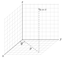
Parameterization of the space with spherical coordinates

${\displaystyle {\begin{aligned}{\frac {\partial v_{1}}{\partial t}}+v_{1}{\frac {\partial v_{1}}{\partial x_{1}}}+v_{2}{\frac {\partial v_{1}}{\partial x_{2}}}+{\frac {1}{\rho }}{\frac {\partial p}{\partial x_{1}}}&=k_{1}\\{\frac {\partial v_{2}}{\partial t}}+v_{1}{\frac {\partial v_{2}}{\partial x_{1}}}+v_{2}{\frac {\partial v_{2}}{\partial x_{2}}}+{\frac {1}{\rho }}{\frac {\partial p}{\partial x_{2}}}&=k_{2}\;.\end{aligned}}}$

In cylindrical coordinates the equations write

${\displaystyle {\begin{array}{rcl}\rho \left({\frac {\mathrm {D} v_{R}}{\mathrm {D} t}}-{\frac {v_{\varphi }^{2}}{R}}\right)&=&-{\frac {\partial p}{\partial R}}+k_{R}\\\rho \left({\frac {\mathrm {D} v_{\varphi }}{\mathrm {D} t}}-{\frac {v_{R}v_{\varphi }}{R}}\right)&=&-{\frac {1}{R}}{\frac {\partial p}{\partial \varphi }}+k_{\varphi }\\\rho {\frac {\mathrm {D} v_{z}}{\mathrm {D} t}}&=&-{\frac {\partial p}{\partial z}}+k_{z}\\{\frac {\mathrm {D} }{\mathrm {D} t}}&:=&{\frac {\partial }{\partial t}}+v_{R}{\frac {\partial }{\partial R}}+{\frac {v_{\varphi }}{R}}{\frac {\partial }{\partial \varphi }}+v_{z}{\frac {\partial }{\partial z}}\end{array}}}$

The operator forms the substantial derivative and the radial coordinate has been marked with instead of in order to avoid confusion with the density. In spherical coordinates we get: ${\displaystyle \mathrm {D} /\mathrm {D} t}$ ${\displaystyle R}$ ${\displaystyle \rho }$

${\displaystyle {\begin{array}{rcl}\rho \left({\frac {\mathrm {D} v_{r}}{\mathrm {D} t}}-{\frac {v_{\varphi }^{2}+v_{\theta }^{2}}{r}}\right)&=&-{\frac {\partial p}{\partial r}}+k_{r}\\\rho \left({\frac {\mathrm {D} v_{\varphi }}{\mathrm {D} t}}+{\frac {v_{r}v_{\varphi }+v_{\theta }v_{\varphi }\cot \theta }{r}}\right)&=&-{\frac {1}{r\sin \theta }}{\frac {\partial p}{\partial \varphi }}+k_{\varphi }\\\rho \left({\frac {\mathrm {D} v_{\theta }}{\mathrm {D} t}}+{\frac {v_{r}v_{\theta }-v_{\varphi }^{2}\cot \theta }{r}}\right)&=&-{\frac {1}{r}}{\frac {\partial p}{\partial \theta }}+k_{\theta }\\{\frac {\mathrm {D} }{\mathrm {D} t}}&:=&{\frac {\partial }{\partial t}}+v_{r}{\frac {\partial }{\partial r}}+{\frac {v_{\varphi }}{r\sin \theta }}{\frac {\partial }{\partial \varphi }}+{\frac {v_{\theta }}{r}}{\frac {\partial }{\partial \theta }}\end{array}}}$

Flow formulation

The above equation of motion is equivalent to the balance equation of the momentum density for ideal fluids with negligible acceleration due to the continuity equation : ${\displaystyle {\vec {k}}}$ ${\displaystyle {\vec {m}}=\rho {\vec {v}}}$

${\displaystyle {\frac {\partial {\vec {m}}}{\partial t}}+\operatorname {div} ({\vec {v}}\otimes {\vec {m}})+\operatorname {grad} (p)={\vec {0}}}$

or in alternative notation

${\displaystyle {\frac {\partial {\vec {m}}}{\partial t}}+\operatorname {div} ({\vec {v}}\otimes {\vec {m}}+p\mathbf {I} )={\vec {0}}\;.}$

The arithmetic symbol " " forms the dyadic product . The symmetric tensor ${\displaystyle \otimes }$

${\displaystyle {\vec {v}}\otimes {\vec {m}}={\vec {m}}\otimes {\vec {v}}=\rho {\vec {v}}\otimes {\vec {v}}=\sum _{i,j=1}^{3}v_{i}m_{j}{\hat {e}}_{i}\otimes {\hat {e}}_{j}}$

is the convective transport of the momentum density , its divergence

${\displaystyle \operatorname {div} ({\vec {v}}\otimes {\vec {m}})=\operatorname {div} ({\vec {v}}){\vec {m}}+\operatorname {grad} ({\vec {m}})\cdot {\vec {v}}}$

is the convective momentum flow .

If one integrates over a fixed volume and applies the Gaussian integral theorem , one obtains: ${\displaystyle V}$

${\displaystyle {\frac {\partial }{\partial t}}\int _{V}{\vec {m}}\;\mathrm {d} V+\oint _{S}({\vec {v}}\otimes {\vec {m}}+p\mathbf {I} )\cdot {\vec {n}}\;\mathrm {d} S={\vec {0}}\;.}$

Here the volume is with the surface and is the normal unit vector on the surface element . This formulation of the equation proves that the momentum is maintained when the static pressure is introduced . The pressure is a surface force and influences the momentum through exchange with the environment. Forces are only transmitted perpendicular to the surface, there are no frictional forces. ${\displaystyle V}$ ${\displaystyle S}$ ${\displaystyle {\vec {n}}}$ ${\displaystyle \mathrm {d} S}$ ${\displaystyle p}$

Conversely, the Euler equations follow from the momentum balance at arbitrary, sufficiently smoothly edged volumes , if one assumes that there is a hydrostatic pressure and only this transfers forces to (and that over the surface and only in the normal direction) - provided the functions that occur are sufficiently smooth to be able to apply the Gaussian integral theorem. ${\displaystyle V}$ ${\displaystyle V}$

Complete system of equations

The above momentum equation does not represent a closed system (even with suitable boundary and initial conditions ). You can already see this intuitively, since in the -dimensional one only has differential equations for unknown functions (speed and pressure). At least one more equation is required to close the system. ${\displaystyle n}$ ${\displaystyle n}$ ${\displaystyle n+1}$

Incompressible case

The assumption of incompressibility is often a sensible approximation for liquids at moderate pressures and for gas flows well below the speed of sound. Incompressible fluids are density-stable ( ) and the equation system is given by adding the conservation of mass in the form of the continuity equation ${\displaystyle \rho ={\text{const.}}}$

${\displaystyle \operatorname {div} {\vec {v}}=0}$

closed. The solution of the equations is simplified by the fact that the pressure can be eliminated from the Euler equation by forming the rotation :

${\displaystyle {\begin{aligned}{\frac {\partial }{\partial t}}\operatorname {rot} ({\vec {v}})+\operatorname {rot(grad} ({\vec {v}})\cdot {\vec {v}})+{\frac {1}{\rho }}\underbrace {\operatorname {rot(grad} (p))} _{={\vec {0}}}=&{\frac {\partial }{\partial t}}\operatorname {rot} ({\vec {v}})+\underbrace {\operatorname {rot} \left({\frac {1}{2}}\operatorname {grad} ({\vec {v}}\cdot {\vec {v}})\right)} _{={\vec {0}}}-\operatorname {rot} ({\vec {v}}\times \operatorname {rot} {\vec {v}})=\operatorname {rot} ({\vec {k}})\\\rightarrow {\frac {\partial }{\partial t}}\operatorname {rot} ({\vec {v}})=&\operatorname {rot} ({\vec {v}}\times \operatorname {rot} ({\vec {v}}))+\operatorname {rot} ({\vec {k}})\,.\end{aligned}}}$

Here, the Grassmann development was used and made use of the fact that gradient fields are always free of rotation.

In the case of incompressibility, the pressure is not calculated from an equation of state of the form but solely from the momentum balance in the form of the Euler equation and the boundary conditions, i.e. H. from the already calculated speed field. Applying the divergence to the Euler equation yields the determining equation for the pressure: ${\displaystyle p=p(\rho )}$

${\displaystyle {\begin{aligned}{\frac {\partial }{\partial t}}\underbrace {\operatorname {div} ({\vec {v}})} _{=0}+\operatorname {div(grad} ({\vec {v}})\cdot {\vec {v}})+{\frac {1}{\rho }}\underbrace {\operatorname {div(grad} (p))} _{=\Delta p}=&\operatorname {div} (\operatorname {grad} ({\vec {v}}))\cdot {\vec {v}}+\operatorname {Sp(grad} ({\vec {v}})\cdot \operatorname {grad} ({\vec {v}}))+{\frac {1}{\rho }}\Delta p\\=&\operatorname {grad} (\underbrace {\operatorname {div} ({\vec {v}})} _{=0})\cdot {\vec {v}}+\operatorname {Sp(grad} ({\vec {v}})\cdot \operatorname {grad} ({\vec {v}}))+{\frac {1}{\rho }}\Delta p=\operatorname {div} ({\vec {k}})\\\rightarrow \Delta p=&\rho \operatorname {div} ({\vec {k}})-\rho \operatorname {Sp(grad} ({\vec {v}})\cdot \operatorname {grad} ({\vec {v}}))\,.\end{aligned}}}$

The operator calculates the track and the product of the velocity gradients is formed with the tensor product " ". In Cartesian coordinates it develops: ${\displaystyle \operatorname {Sp} }$ ${\displaystyle \cdot }$

${\displaystyle \operatorname {Sp(grad} ({\vec {v}})\cdot \operatorname {grad} ({\vec {v}}))=\operatorname {Sp} \left(\sum _{i,j=1}^{3}{\frac {\partial {\vec {v}}}{\partial x_{i}}}\otimes {\hat {e}}_{i}\cdot {\frac {\partial {\vec {v}}}{\partial x_{j}}}\otimes {\hat {e}}_{j}\right)=\operatorname {Sp} \left(\sum _{i,j=1}^{3}{\frac {\partial v_{i}}{\partial x_{j}}}{\frac {\partial {\vec {v}}}{\partial x_{i}}}\otimes {\hat {e}}_{j}\right)=\sum _{i,j=1}^{3}{\frac {\partial v_{i}}{\partial x_{j}}}{\frac {\partial v_{j}}{\partial x_{i}}}\,.}$

Compressible case

In the case of compressible fluids, and particularly when temperature is another unknown, one also needs the conservation of energy and equations of state (i.e., constitutive equations ) of the fluid to be modeled. In the three-dimensional case, the five coupled differential equations result

${\displaystyle {\frac {\partial {\vec {u}}}{\partial t}}+\left(\operatorname {div} \mathbf {f} \left({\vec {u}}\right)\right)^{\top }={\vec {0}}\;,}$

where is the vector of the conservation variable and the flow with enthalpy is given by the following expressions: ${\displaystyle {\vec {u}}=\left(\rho ,\,\rho v_{1},\,\rho v_{2},\,\rho v_{3},\,\rho H\right)^{\top }}$ ${\displaystyle \mathbf {f} =\left({\vec {f}}_{1},\,{\vec {f}}_{2},\,{\vec {f}}_{3}\right)^{\top }}$ ${\displaystyle H}$

${\displaystyle {\vec {f}}_{1}={\begin{pmatrix}\rho v_{1}\\\rho v_{1}^{2}+p\\\rho v_{1}v_{2}\\\rho v_{1}v_{3}\\\rho v_{1}H\end{pmatrix}}\,,\quad {\vec {f}}_{2}={\begin{pmatrix}\rho v_{2}\\\rho v_{1}v_{2}\\\rho v_{2}^{2}+p\\\rho v_{2}v_{3}\\\rho v_{2}H\end{pmatrix}}\,,\quad {\vec {f}}_{3}={\begin{pmatrix}\rho v_{3}\\\rho v_{1}v_{3}\\\rho v_{2}v_{3}\\\rho v_{3}^{2}+p\\\rho v_{3}H\end{pmatrix}}\;.}$

The first equation in this system is the continuity equation for the compressible case

${\displaystyle {\frac {\partial \rho }{\partial t}}+\operatorname {div} \left(\rho \,{\vec {v}}\right)=0\;,}$

the second to fourth equations are the momentum equations (Euler equations in the narrower sense, see above) and the last equation is the energy balance. Together with a thermal equation of state, which links pressure , temperature and density , and a caloric equation of state, which links temperature , pressure and enthalpy , one obtains a formally closed system of equations around the seven unknown quantities speed , and , pressure , density , temperature and Calculate enthalpy . In practice, a perfect gas model is often used; H. an ideal gas with constant specific heat capacity . ${\displaystyle p}$ ${\displaystyle T}$ ${\displaystyle \rho }$ ${\displaystyle T}$ ${\displaystyle p}$ ${\displaystyle H}$ ${\displaystyle v_{1}}$ ${\displaystyle v_{2}}$ ${\displaystyle v_{3}}$ ${\displaystyle p}$ ${\displaystyle \rho }$ ${\displaystyle T}$ ${\displaystyle H}$

In this model, heat conduction and internal friction are neglected. If one also takes into account the effects of friction and possibly heat conduction, the Navier-Stokes equations for compressible fluids are obtained instead of the Euler equations .

boundary conditions

A condition on solid walls is that the velocity in the normal direction is zero so that the fluid cannot flow through the wall. On an arbitrary time-dependent shaped surface , by a function will be described and then its normal , it is ${\displaystyle {\vec {n}}}$ ${\displaystyle {\vec {n}}\cdot {\vec {v}}=0\,,}$ ${\displaystyle f({\vec {x}},t)=0}$ ${\displaystyle {\vec {n}}=\operatorname {grad} (f)}$

${\displaystyle {\frac {\partial f({\vec {x}},t)}{\partial t}}+\operatorname {grad} {\bigl (}f({\vec {x}},t){\bigr )}\cdot {\vec {v}}({\vec {x}},t)=0}$

for all set on the edge of the fluid. Because of the assumed freedom from friction, no condition is placed on the tangential component of the speed, which is in contrast to the Navier-Stokes equations, in which the no-slip condition applies. ${\displaystyle {\vec {x}}}$

In addition, pressure boundary conditions, such as on the free surface of a body of water, can occur. Because pressure can only be exerted on material particles, such a surface is a material surface, the substantial time derivative of which therefore disappears and the boundary condition then reads:

${\displaystyle {\frac {\mathrm {D} g({\vec {x}},t)}{\mathrm {D} t}}={\frac {\partial g({\vec {x}},t)}{\partial t}}+\operatorname {grad} {\bigl (}g({\vec {x}},t){\bigr )}\cdot {\vec {v}}({\vec {x}},t)=0\quad {\text{und}}\quad p({\vec {x}},t)=p_{0}({\vec {x}},t)}$

for all on the edge of the fluid, which is described by the function and on which the pressure is specified. The normal component of the velocity generally does not disappear on such surfaces, so that they are carried along by the current, and the determination of the surface is then part of the problem. Mostly, especially in the technical field such as B. at the outlet of a pipe through which there is a flow, the area is known, which considerably simplifies the task. ${\displaystyle {\vec {x}}}$ ${\displaystyle g}$ ${\displaystyle p_{0}}$ ${\displaystyle g}$

Mathematical properties

The Euler equations belong to the class of nonlinear hyperbolic conservation equations. This means that after a finite time, even with smooth initial data, discontinuities such as shocks ( shock waves) occur. Under strong conditions, global smooth solutions exist in the relevant case , for example when the solution moves in a kind of dilution wave. In the stationary case, the equation is elliptical or hyperbolic, depending on the Mach number . In a transonic flow , both subsonic and supersonic regions occur and the equation has a mixed character. ${\displaystyle \rho ,p>0}$

The eigenvalues of the equations are the speed in the normal direction (with multiplicity of dimensions) and this plus minus the speed of sound , . This means that the Euler equations using the ideal gas equation as a pressure function in the one-dimensional are even strictly hyperbolic, so that there are useful existence and uniqueness results for this case. In the multidimensional, they are no longer strictly hyperbolic due to the multiple eigenvalue. This makes the mathematical solution extremely difficult. This is primarily about determining physically meaningful weak solutions , i.e. those that can be interpreted as solutions to the Navier-Stokes equations with vanishing viscosity. ${\displaystyle v_{n}}$ ${\displaystyle v_{n}\pm c}$

In addition to the above-mentioned differences in the boundary conditions and with regard to boundary layer formation, the lack of turbulence is an essential difference between the Euler and Navier-Stokes equations.

The Euler equations are rotationally invariant. In addition, the flow functions are homogeneous, so it applies . ${\displaystyle {\vec {f}}_{l}({\vec {u}})={\frac {\partial {\vec {f}}_{l}({\vec {u}})}{\partial {\vec {u}}}}{\vec {u}}}$

Lars Onsager suspected in 1949 that the Euler equation already shows turbulence phenomena, although there is no internal friction (viscosity) there as with the Navier-Stokes equation. In particular, he hypothesized that the weak solutions of the three-dimensional incompressible Euler equation show a change in behavior at the exponent of Hölder continuity of one third: below there are solutions with anomalous dissipation of the (kinetic) energy (violation of the conservation of energy), above not. The conjecture was proven by Philip Isett in 2017 after preliminary work by a number of mathematicians .

Numerical solution

Since the Euler equations are conservation equations , they are usually solved with the help of finite volume methods . Conversely, efforts in the field of aerodynamics since the 1950s to numerically simulate the Euler equations have been the driving force behind the development of finite volume methods. Since, in contrast to the Navier-Stokes equations, no boundary layer has to be taken into account, the simulation can take place on a comparatively coarse calculation grid . The main difficulty is the treatment of the Euler flow, which is usually treated with the help of approximate Riemann solvers. These provide an approximation to the solution of Riemann problems along cell edges. The Riemann problem of the Euler equations can even be solved exactly, but the calculation of this solution is extremely complex. For this reason, numerous approximate solvers have been developed since the 1980s, starting with the Roe solver up to the AUSM family in the 1990s.

The CFL condition must be observed for the time integration . Especially in the area of ​​Mach numbers close to zero or one, the equations become very stiff due to the different eigenvalue scales, which makes the use of implicit time integration methods necessary: ​​the CFL condition is based on the greatest eigenvalue ( ), while the parts of the flow that are relevant for the simulation move. In most cases, an explicit procedure would therefore require an unacceptably large number of time steps. ${\displaystyle v_{n}\pm c}$ ${\displaystyle v_{n}}$

The solution of the non-linear equation systems that occur is then carried out either with the aid of preconditioned Newton - Krylow methods or with special non - linear multigrid methods .

Special cases

A number of basic gas dynamics equations can be derived from the Euler equations . These include Bernoulli's energy equation mentioned at the beginning and potential flow, to which our own articles are dedicated. In the following, the wave equations of linear acoustics, the conservation of the kinetic energy of the fluid elements in a fixed volume and the flow function in flat, density- stable and stationary flows are presented.

Wave equations of linear acoustics

A gas at rest, in equilibrium, is given, in which the velocity field, density, pressure and temperature are constant in space and time. This denotes the ground state of the gas. Variables are considered whose constant ground state is superimposed with small disturbances , whose local derivatives are also small. The disturbances are also so small and fast that the heat flows can also be neglected (“adiabatic processes”). Then the mass balance is at the point : ${\displaystyle \varphi =\varphi _{0}+\varphi '}$ ${\displaystyle \varphi _{0}}$ ${\displaystyle \varphi '}$ ${\displaystyle {\vec {v}}_{0}={\vec {0}}}$

${\displaystyle {\frac {\partial (\rho _{0}+\rho ')}{\partial t}}+\operatorname {div} [(\rho _{0}+\rho '){\vec {v}}']={\frac {\partial \rho '}{\partial t}}+\operatorname {div} (\rho _{0}{\vec {v}}')+\operatorname {div} (\rho '{\vec {v}}')\approx {\frac {\partial \rho '}{\partial t}}+\rho _{0}\operatorname {div} ({\vec {v}}')=0\,.}$		(I)

The Euler equation takes the form

${\displaystyle {\frac {\partial {\vec {v}}'}{\partial t}}+\operatorname {grad} ({\vec {v}}')\cdot {\vec {v}}'+{\frac {1}{\rho _{0}+\rho '}}\operatorname {grad} (p_{0}+p')\approx {\frac {\partial {\vec {v}}'}{\partial t}}+{\frac {1}{\rho _{0}}}\operatorname {grad} (p')={\vec {k}}}$		(II)

because the quadratic convective acceleration can be neglected compared to the local acceleration. Partial time derivative of the mass balance (I) and subtraction of the multiplied by divergence of the Euler equation (II) yields with divergence-free gravitational acceleration ( ): ${\displaystyle \rho _{0}}$ ${\displaystyle \operatorname {div} \,{\vec {k}}=0}$

${\displaystyle {\begin{aligned}0&={\frac {\partial ^{2}\rho '}{\partial t^{2}}}+\rho _{0}{\frac {\partial }{\partial t}}\operatorname {div} ({\vec {v}}')\\0&=\rho _{0}\operatorname {div} \left({\frac {\partial {\vec {v}}'}{\partial t}}\right)+\underbrace {\operatorname {div} (\operatorname {grad} (p'))} _{=\Delta p'}\\\Rightarrow \quad 0&={\frac {\partial ^{2}\rho '}{\partial t^{2}}}+\underbrace {\rho _{0}{\frac {\partial }{\partial t}}\operatorname {div} ({\vec {v}}')-\rho _{0}\operatorname {div} \left({\frac {\partial {\vec {v}}'}{\partial t}}\right)} _{=0}-\Delta p'={\frac {\partial ^{2}\rho '}{\partial t^{2}}}-\Delta p'\,.\end{aligned}}}$

In an ideal gas, the pressure change under the given conditions is proportional to the change in density , and this is how the wave equations of linear acoustics arise : ${\displaystyle p'=c^{2}\rho '}$

${\displaystyle {\dfrac {\partial ^{2}\rho '}{\partial t^{2}}}=c^{2}\Delta \rho '\quad ,\qquad {\dfrac {\partial ^{2}p'}{\partial t^{2}}}=c^{2}\Delta p'\,.}$

The constant is the speed of sound and is the Laplace operator . ${\displaystyle c}$ ${\displaystyle \Delta }$

Energy conservation

In a conservative gravitational field, the total kinetic energy of the fluid elements remains constant in a fixed volume completely filled with an incompressible fluid. The fluid cannot come to rest because

1. there is no dissipation mechanism in the form of internal friction ( viscosity ) or friction on the walls in the Euler equations ,
2. a conversion of the kinetic energy into position energy is not possible because of the completely filled volume and the constant density in the sum and because
3. the kinetic energy cannot do compression work because of the incompressibility.

proof0

To prove this, it must first be established that in an incompressible fluid the divergence of the velocity disappears and the density is constant. So the Euler equations read in a conservative gravitational field with : ${\displaystyle {\vec {k}}=-\operatorname {grad} V}$ ${\displaystyle {\frac {\partial {\vec {v}}}{\partial t}}+\operatorname {grad} ({\vec {v}})\cdot {\vec {v}}=:{\dot {\vec {v}}}=-{\frac {1}{\rho }}\operatorname {grad} p+{\vec {k}}=-\operatorname {grad} \left({\frac {p}{\rho }}+V\right)=:\operatorname {grad} \,B\,.}$ The added point denotes the substantial time derivative . From the total kinetic energy ${\displaystyle E_{\mathrm {kin} }:=\int _{v_{0}}{\frac {1}{2}}{\vec {v}}\cdot {\vec {v}}\,\mathrm {d} v}$ the time derivative is taken in the fixed volume , which is easily possible due to the fixed integration limits: ${\displaystyle v_{0}}$ ${\displaystyle {\frac {\mathrm {d} }{\mathrm {d} t}}E_{\mathrm {kin} }={\frac {\mathrm {d} }{\mathrm {d} t}}\int _{v_{0}}{\frac {1}{2}}({\vec {v}}\cdot {\vec {v}})\,\mathrm {d} v=\int _{v_{0}}{\dot {\vec {v}}}\cdot {\vec {v}}\,\mathrm {d} v=\int _{v_{0}}\operatorname {grad} (B)\cdot {\vec {v}}\,\mathrm {d} v}$ The last term integrates the power of the pressure and the gravitational field, which is equal to the change in kinetic energy. In an incompressible fluid, due to the product rule: ${\displaystyle \operatorname {div} (B{\vec {v}})=\operatorname {grad} (B)\cdot {\vec {v}}+B\operatorname {div} {\vec {v}}=\operatorname {grad} (B)\cdot {\vec {v}}\,.}$ This means that because of neither the pressure nor the gravity field can do compression work. Exploitation of the Gaussian integral theorem and the fact that in a rigidly bordered volume the normal component of the velocity disappears at the edge of the volume, yields the desired: ${\displaystyle \operatorname {div} {\vec {v}}=0}$ ${\displaystyle {\vec {v}}\cdot \,\mathrm {d} {\vec {a}}}$ ${\displaystyle \partial v_{0}}$ ${\displaystyle {\frac {\mathrm {d} }{\mathrm {d} t}}E_{\mathrm {kin} }=\int _{v_{0}}\operatorname {grad} (B)\cdot {\vec {v}}\,\mathrm {d} v=\int _{v_{0}}\operatorname {div} (B{\vec {v}})\,\mathrm {d} v=\int _{\partial v_{0}}B{\vec {v}}\cdot \,\mathrm {d} {\vec {a}}=0\,.}$

Flat and steady flow of an incompressible fluid

→ Main article : Electricity function

A stationary flow taking place in the xy plane is considered. The condition for incompressibility is then in Cartesian coordinates ${\displaystyle \operatorname {div} {\vec {v}}=0}$

${\displaystyle {\frac {\partial v_{x}}{\partial x}}+{\frac {\partial v_{y}}{\partial y}}=0}$

and is fulfilled identically if the velocity components are derived from the derivatives of a scalar function according to

${\displaystyle v_{x}={\frac {\partial \psi }{\partial y}}\,,\quad v_{y}=-{\frac {\partial \psi }{\partial x}}}$

to calculate. The function is called the current function . The value of the current function is constant along a streamline, so that its contour lines represent streamlines. Its contour lines are closed curves in the vicinity of extreme points of the flow function. A maximum of the flow function is counterclockwise, a minimum is clockwise. ${\displaystyle \psi }$

See also

• Vertebral sets
• Speed ​​potential
• Tensoranalysis formula collection

literature

• LD Landau, EM Lifschitz: Textbook of Theoretical Physics, Volume VI Hydrodynamics. Akademie Verlag, Berlin 1991, ISBN 3-05-500070-6 .
• Ralf Greve: Continuum Mechanics . Springer, 2003, ISBN 3-540-00760-1 .
• M. Bestehorn: hydrodynamics and structure formation . Springer, 2006, ISBN 978-3-540-33796-6 .
• GK Batchelor : An introduction to Fluid Dynamics. (= Cambridge mathematical library ). Cambridge University Press, Cambridge u. a. 2000, ISBN 0-521-66396-2 .
• Alexandre Chorin , Jerrold Marsden : A Mathematical Introduction to Fluid Mechanics. (= Texts in Applied Mathematics. 4). 3rd edition corrected, 3rd printing. Springer, New York NY a. a. 1998, ISBN 3-540-97918-2 .
• Pierre-Louis Lions : Mathematical Topics in Fluid Mechanics. Volume 1: Incompressible Models. (= Oxford lecture series in mathematics and its applications. 3). Clarendon Press, Oxford et al. a. 1996, ISBN 0-19-851487-5 .
• Pierre-Louis Lions: Mathematical Topics in Fluid Mechanics. Volume 2: Compressible Models. (= Oxford lecture series in mathematics and its applications. 10). Clarendon Press, Oxford et al. a. 1998, ISBN 0-19-851488-3 .
• Edwige Godlewski, Pierra-Arnaud Raviart: Hyperbolic Systems of Conservation Laws. (= Mathématiques & applications. 3/4). Ellipses, Paris 1991.

Footnotes

1. ↑ where denotes the cross product . ${\displaystyle \operatorname {grad} ({\vec {v}})\cdot {\vec {v}}={\frac {1}{2}}\operatorname {grad} ({\vec {v}}\cdot {\vec {v}})-{\vec {v}}\times \operatorname {rot} ({\vec {v}})}$ ${\displaystyle \times }$
2. ↑ The product rule is used , where is here . The operator Sp calculates the track . The identity applies to all vector fields . In the literature there are other definitions of the divergence operator for tensors, which differ from the one used here by the transposition of their argument. Deviating formulas for the derivation cannot be ruled out in the literature. ${\displaystyle \operatorname {div} (\mathbf {T} \cdot {\vec {v}})=\operatorname {div} (\mathbf {T} )\cdot {\vec {v}}+\operatorname {Sp} (\mathbf {T} \cdot \operatorname {grad} ({\vec {v}}))}$ ${\displaystyle \mathbf {T} =\operatorname {grad} ({\vec {v}})}$ ${\displaystyle \operatorname {div(grad} ({\vec {v}}))=\operatorname {grad(div} ({\vec {v}}))}$ ${\displaystyle {\vec {v}}}$

Individual evidence

1. ^ M. Bestehorn: hydrodynamics and structure formation. 2006, p. 52.
2. ^ M. Bestehorn: hydrodynamics and structure formation. 2006, p. 380 ff.
3. ^ M. Bestehorn: hydrodynamics and structure formation. 2006, p. 54.
4. ↑ P. Haupt: Continuum Mechanics and Theory of Materials . Springer, 2002, ISBN 3-540-43111-X , pp. 179 ff .
5. ↑ Ralf Greve: Continuum Mechanics. 2003, p. 146 ff.
6. ↑ C. Marchioro, M. Pulvirenti: Mathematical theory of incompressible fluids nonviscous . Springer, 1994, ISBN 3-540-94044-8 , pp. 23 f .