
Grid (geometry)
A grid in geometry is a gapless and overlap-free partition of a space by a set of grid cells . The grid cells are defined by a set of grid points that are connected to one another by a set of grid lines .
Grids are used in science and technology for surveying , modeling and numerical calculations (see grid model ).
Classification
Grids are divided into different categories based on their topology and geometry. A fundamental distinction is made between structured and unstructured grids.
Textured grid


Structured grids (English structured grids ) have a regular topology, but not necessarily a regular cell geometry. With structured grids, the cells are in a regular grid so that the cells can be clearly indexed using whole numbers. One-dimensional grids (line grids) are always structured, the cells can be counted through i = 1..N (N = number of elements). For two-dimensional grids an element is uniquely determined by the indices (i, j), for three-dimensional grids by the indices (i, j, k). The advantage of using structured grids over the unstructured grids described below is that this unique indexing allows neighboring cells to be determined without computational effort. Structured grids always consist of one element type. Rectangular elements are mostly used in two-dimensional and triangular elements only rarely. Three-dimensional lattices are almost always hexahedra and only sometimes tetrahedra . The use of triangular elements or tetrahedra has the disadvantage that they only poorly fill the space and more elements are necessary. For example, a tetrahedron with an edge length of 1 only has a volume of 1/6, while a cube has a volume of 1. Therefore, for the flow simulation, for example, tetrahedral grids have to use a large number of cells in order to achieve sufficient resolution.
In the case of the structured grids, complex structures are also possible in which the grid system is regular, but overall curved or adapted to a complex geometry. Multiblock structures are also used, in which the grid is formed from several structured blocks of different sizes. Such structured grids can only be created partially automatically.
In the case of curved grids (English curvilinear grids ), the grid lines are given by parameterized curves. However, the term is rather uncommon. One then speaks simply of structured grids.
Right-angled grids (English rectilinear grids ) divide the space completely into axially parallel areas that do not have to be the same size. In three-dimensional space, cuboids of different or the same size are created.
A regular grid (English regular grid ) divides the space completely in axis-parallel rectangular portions, said edges along an axis always have the same length.
The simplest case is a Cartesian grid (English Cartesian grid ) in which all edge lengths are equal. In two-dimensional space, a square area is created and in three-dimensional space, a volume of cubes.
Unstructured grid

Unstructured grids (English unstructured grids ) have no set topology and no uniform grid cell geometry. Unstructured grids are mostly the result of an adaptation process. Also known are grids made of complex cells, so-called polyhedral grids. The cell structure here is similar to that of soap foam.
Unstructured grids can be used very flexibly and can also be easily generated automatically. However, data management is more complex than with structured grids. On the one hand, the grid points are not arranged in a regular pattern as is the case with structured grids, but have to be saved individually. On the other hand, it is not clear from the start which cells are neighboring to a particular grid cell. This neighborhood information must either be stored explicitly when the grid is generated or it must be calculated in a complex manner at runtime. Unstructured grids therefore generally require a multiple of the memory requirements of structured grids and generally cause a higher computational effort.
Grid generation
As mesh generation or Meshing refers to a group of procedures in computer graphics , as well as the simulation of the physical properties of solids and fluids; In this process, a given surface or a given volume of space is approximated ( approximated ) by a number of smaller, mostly very simple elements . The resulting grid is a simplified description of the surface or the body, which then z. B. can be used for further calculations, for example by means of the finite element method (FEM).
In the case of two-dimensional surfaces, triangular or quadrangular elements are most often used to generate the grid , while three-dimensional bodies usually use tetrahedra or cuboids .
The generation of a grid of triangular elements is also called triangulation (or triangulation ) referred to (as well as the resulting triangular lattice), the generation of a grid of square elements is also Paving . If the number of outer edges of a surface is fixed and the number is odd, then pure square paving is not possible (at least one element remains with an odd number of corners, e.g. a triangle).
Triangular grid
In trigonometry and elementary geometry, the division of a surface into triangles is referred to as a triangular grid , triangular network or triangulation . In terms of graph theory , triangular grids are of the type “undirected graphs without multiple edges”, whose subgraphs are “ circles with three nodes ” (and correspondingly three edges ). The generalization of triangle meshes are polygon meshes .
A triangulation of a set of points in the plane denotes a division of the convex envelope of the set of points into triangles, the corner points of the triangles being exactly the points from . Thus the triangulation is a planar triangle graph . If the set is in a convex position, the number of possible triangulations is exactly the -th Catalan number , where the number of points denotes in.


One is often interested in calculating a triangulation with special properties. For example there is the Delaunay triangulation , which maximizes the smallest interior angle of the triangles, or the minimum weight triangulation , which minimizes the total length of all edges.
Adaptive grids

A distinction is also made between adaptive and non-adaptive discretizations.
Non-adaptive gratings have the same resolution everywhere. In the case of small geometric structures or areas with strong curves, acute angles or differently defined material parameters, a coarse grid with large grid cells is no longer sufficient to discretize such problem areas with sufficient accuracy. A global refinement of the grid is mostly not useful because of the associated increased storage and computing time.
Here, the method accesses the adaptive mesh generation (English adaptive meshing ), which, when large errors are expected to select the fine grid. This is done either through a priori knowledge of the problem under consideration or through methods that use given error estimates to dynamically refine where the error is currently large. The latter is particularly important in the case of transient problems, i.e. if the problematic areas change their position over time.
Another method for discretizing critical areas is sub-grid technology .
Applications
technology
- In technical design for the modeling of curved surfaces, especially in connection with CAD (CAD)
- In robotics for determining joint positions; this results in highly dynamic triangular networks that reflect the movement
- In the building industry for the measurement of a structure with triangles: Here triangular nets - especially right-angled (3: 4: 5) and equilateral - were already common in gothic construction huts . Modern applications are CAM processes
Surveying
- In geodesy as a surveying network for determining points, see Triangulation (Geodesy) : Trigonometric points (TP) are measured as surveying points using the network
- For photogrammetry to record the data - with line-by-line scanning, square meshes are more common (but they can easily be converted into triangular meshes in order to make them accessible to the specific algorithms)
- In GIS technology and other satellite-based measurement methods for converting the mostly linear measurement series to an earth model
numerical Mathematics
In numerical mathematics, a computational grid is a discrete decomposition of the space on which a partial differential equation is to be solved. The term is not used for a temporal discretization . The intersections of two grid lines are called nodes, the cells either as cells, in finite element methods also as elements and in finite volume methods as volumes. The grid can be spatially fixed or move over time or be adapted in the course of the calculation.
At the edges of the area, boundary conditions must be specified.
Computational grids do not have to be one-dimensional. With three-dimensional grids, very large numbers of cells are quickly reached. A simple right-angled grid that resolves only 100 cells on one edge already has 1 million cells in the third dimension .
On modern PCs with 2 GB main memory, approx. 1.5–5 million cells can be calculated today, depending on the software system. If larger resolutions are required, the calculation must be carried out on mainframes or computer networks .
Examples
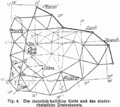
Geodetic survey network
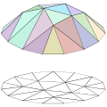
Lattice generation in computer graphics

Flat triangular mesh for FEM modeling
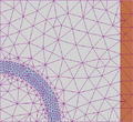
Adaptive planar triangular mesh for FEM modeling


literature
- Michael Bender, Manfred Brill: Computer graphics - An application-oriented textbook . 2nd Edition. Hanser, 2006, ISBN 3-446-40434-1 .
- Hansen and Johnson: The Visualization Handbook . Elsevier, Burlington 2005, ISBN 0-12-387582-X .