Current function

The flow function (symbol , dimension L² T ⁻¹ ) is an analytical aid in fluid mechanics for solving the equations of motion in flat, stationary flows of incompressible fluids . The assumption of incompressibility is often a sensible approximation for liquids at moderate pressures and for gas flows well below the speed of sound. The velocity field results from the derivatives of the current function, which is then automatically divergence-free as in the case of an incompressible fluid. The contour lines on which the value of the current function is constant represent streamlines , which is what gives this function its name. The concept of the current function can also be applied to axially symmetrical flows in the form of Stokes' current function . ${\displaystyle \psi }$

Is the flow viscosity - and irrotational as in potential flow , then the current function of the imaginary part of the complex velocity potential . This article does not require the flow to be viscous or free from turbulence.

definition

A level, density-stable and steady flow with a location-dependent but not time-dependent because it is stationary velocity field is considered. The unit vector is perpendicular to the plane through which the flow passes. ${\displaystyle {\vec {v}}({\vec {x}})\,.}$ ${\displaystyle {\hat {e}}_{z}}$

Then the current function is a function from which the velocity with the derivatives ${\displaystyle \psi }$

${\displaystyle {\vec {v}}=\operatorname {rot} (\psi {\hat {e}}_{z})=\operatorname {grad} (\psi )\times {\hat {e}}_{z}\quad \Rightarrow \quad v_{x}={\frac {\partial \psi }{\partial y}}\,,\quad v_{y}=-{\frac {\partial \psi }{\partial x}}\,.}$

calculated. The operators “red” and “grad” stand for the rotation or the gradient and the arithmetic symbol “×” forms the cross product . The equation on the left is independent of the coordinate system selected in the plane, while the equation on the right presupposes a Cartesian coordinate system in which the speed component is in the x-direction and that in the y-direction. ${\displaystyle v_{x}}$ ${\displaystyle v_{y}}$

Properties of flows described with stream functions

Streamlines

The gradient of the current function is due to

${\displaystyle \operatorname {grad} (\psi )\cdot {\vec {v}}=\operatorname {grad} (\psi )\cdot (\operatorname {grad} (\psi )\times {\hat {e}}_{z})=0}$

perpendicular to the speed. The speed is by definition tangential to it on any streamline, so the value of the stream function does not change on a streamline. This is also calculated from the definition of the streamline and one of its line elements for which by definition or equivalent, the following applies: ${\displaystyle \mathrm {d} {\vec {x}}={\vec {v}}\mathrm {d} t\,,}$ ${\displaystyle {\vec {v}}\parallel \mathrm {d} {\vec {x}}}$ ${\displaystyle {\vec {v}}\times \mathrm {d} {\vec {x}}={\vec {0}}}$

${\displaystyle {\begin{aligned}{\vec {v}}\times \mathrm {d} {\vec {x}}=(\operatorname {grad} (\psi )\times {\hat {e}}_{z})\times \mathrm {d} {\vec {x}}=(\operatorname {grad} (\psi )\cdot \mathrm {d} {\vec {x}}){\hat {e}}_{z}=\mathrm {d} \psi {\hat {e}}_{z}=&{\vec {0}}\\\Rightarrow \quad \mathrm {d} \psi ={\frac {\partial \psi }{\partial x}}\mathrm {d} x+{\frac {\partial \psi }{\partial y}}\mathrm {d} y=&0\,.\end{aligned}}}$

The value of the current function is therefore constant along a streamline.

Critical points of the current function

At critical points of the current function, its gradient disappears, the components of which are the velocity components. So there is a standstill in the critical points of the current function. Because of the sticking condition , this is the case everywhere in linear-viscous fluids on walls. Therefore, only critical points in the fluid apart from walls are considered. If the critical point is an extreme point (not a saddle point ), then the contour lines of the flow function, i.e. the flow lines, are closed curves in its vicinity. A maximum of the flow function is counterclockwise, a minimum is clockwise.

Density stability

If the velocity field of a plane flow is given by a flow function, then:

${\displaystyle \operatorname {div} {\vec {v}}=\operatorname {div(rot} (\psi {\hat {e}}_{z}))=0\,,}$

because every field of rotation is divergence-free. The operator “div” calculates the divergence of a vector field . In a divergence-free flow, due to the mass balance, the substantial time derivative of the density disappears everywhere , which is therefore at least constant over time. In an incompressible fluid, the density is also spatially constant and the flow field is in any case free of divergence. The assumption of incompressibility is often a sensible approximation for liquids at moderate pressures and for gas flows well below the speed of sound.

A divergence-free flow contains neither sources nor sinks, so that under the given conditions streamlines in the interior of the liquid can neither begin nor end. The streamlines are either closed or run to the edge.

Rotation of the flow

The rotation of the velocity field has only one component perpendicular to the plane in the plane case:

${\displaystyle \operatorname {rot} {\vec {v}}=\operatorname {rot(grad} (\psi )\times {\hat {e}}_{z}))=\operatorname {grad} (\operatorname {grad} (\psi ))\cdot {\hat {e}}_{z}-\operatorname {div} (\operatorname {grad} (\psi )){\hat {e}}_{z}=-\Delta \psi {\hat {e}}_{z}\,,}$

because the derivation of the current function perpendicular to the plane disappears and thus also its gradient in this direction. The symbol “ ” denotes the Laplace operator . Especially in Cartesian coordinates the following is calculated: ${\displaystyle \Delta }$

${\displaystyle \operatorname {rot} {\vec {v}}=\left({\frac {\partial v_{y}}{\partial x}}-{\frac {\partial v_{x}}{\partial y}}\right){\hat {e}}_{z}=\left(-{\frac {\partial ^{2}\psi }{\partial x^{2}}}-{\frac {\partial ^{2}\psi }{\partial y^{2}}}\right){\hat {e}}_{z}=-\Delta \psi {\hat {e}}_{z}\,.}$

In eddy-free flows, such as potential flows, the Laplace equation applies.As announced at the beginning, this will not be discussed any further at this point, but reference is made to the articles on velocity potential and potential flow. ${\displaystyle \Delta \psi =0\,.}$

Volume flow between streamlines

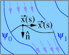
The volume flow that occurs between two streamlines over the black line is independent of the location and the course of the line

The volume flow between two streamlines is the same everywhere. This is shown using two streamlines, on which the current function assumes the values ψ ₀ and ψ ₁ . To calculate the volume flow that passes between these two streamlines, a line with the arc length and is defined, which therefore begins on one streamline and ends on the other streamline, see picture. The parameterization with the arc length causes l is the length of the curve and the amount Tangentenvekor one has: The volume flow which passes over the line, calculated with a line integral of the curve and the normal to ${\displaystyle {\vec {x}}(s)}$ ${\displaystyle s\in [0,l]\,,\;\psi ({\vec {x}}(0))=\psi _{0}}$ ${\displaystyle \psi ({\vec {x}}(l))=\psi _{1}}$ ${\displaystyle |{\vec {x}}'(s)|=1\,.}$ ${\displaystyle {\dot {v}}_{01}}$ ${\displaystyle {\hat {n}}={\vec {x}}'\times {\hat {e}}_{z}}$

${\displaystyle {\begin{aligned}{\dot {v}}_{01}=&\int _{0}^{l}{\vec {v}}\cdot {\hat {n}}\mathrm {d} s=\int _{0}^{l}(\operatorname {grad} (\psi )\times {\hat {e}}_{z})\cdot {\hat {n}}\mathrm {d} s=\int _{0}^{l}(\underbrace {{\hat {e}}_{z}\times {\hat {n}}} _{{\vec {x}}'})\cdot \operatorname {grad} (\psi )\mathrm {d} s\\=&\int _{0}^{l}\operatorname {grad} (\psi )\cdot \underbrace {{\vec {x}}'\mathrm {d} s} _{=\mathrm {d} {\vec {x}}}=\int _{{\vec {x}}(0)}^{{\vec {x}}(l)}\operatorname {grad} (\psi )\cdot \mathrm {d} {\vec {x}}=\int _{\psi _{0}}^{\psi _{1}}\mathrm {d} \psi =\psi _{1}-\psi _{0}\,.\end{aligned}}}$

Regardless of the specific curve shape, the volume flow between two streamlines is the same everywhere. If the line starts and ends on the same streamline, the volume flow across it disappears. If the selected line is part of a streamline, then it will be seen that at no point in a streamline does fluid flow over it. A streamline acts like an impenetrable wall.

Determining equations for the current function

Not every flow function represents a physically realistic flow. In order for the current function to be in accordance with the laws of physics, it must obey the Euler equations with no viscosity and the Navier-Stokes equations with linear viscosity , from which - as can be seen - the current function can be calculated independently of the pressure. In a conservative gravitational field, the search for the current function is particularly easy. The pressure in the fluid can then be derived from the flow function.

Viscosity-free fluids

The Euler equations provide an equation for the current function by forming the rotation:

${\displaystyle {\begin{aligned}\operatorname {rot} \left(\operatorname {grad} ({\vec {v}})\cdot {\vec {v}}+{\frac {1}{\rho }}\operatorname {grad} (p)\right)=&\operatorname {rot} ({\vec {k}})\\\Rightarrow \quad [\operatorname {grad} (\psi )\times \operatorname {grad} (\Delta \psi )]\cdot {\hat {e}}_{z}=&\operatorname {rot} ({\vec {k}})\cdot {\hat {e}}_{z}\,.\end{aligned}}}$

The last equation must satisfy the flow function in order to describe a physically realistic flow.

proof

Exploitation of the Grassmann development ${\displaystyle \operatorname {grad} ({\vec {v}})\cdot {\vec {v}}={\frac {1}{2}}\operatorname {grad} ({\vec {v}}\cdot {\vec {v}})-{\vec {v}}\times \operatorname {rot} ({\vec {v}})}$ shows in the formation of the rotation in the Euler equations: ${\displaystyle {\begin{aligned}\operatorname {rot} {\vec {k}}=&\operatorname {rot} \left(\operatorname {grad} ({\vec {v}})\cdot {\vec {v}}+{\frac {1}{\rho }}\operatorname {grad} (p)\right)=\operatorname {rot} \left({\frac {1}{2}}\operatorname {grad} ({\vec {v}}\cdot {\vec {v}})-{\vec {v}}\times \operatorname {rot} ({\vec {v}})\right)\\=&\operatorname {rot(rot} ({\vec {v}})\times {\vec {v}})\,,\end{aligned}}}$ because gradient fields are always free of rotation. With the product rule ${\displaystyle \operatorname {rot} ({\vec {f}}\times {\vec {g}})=\operatorname {grad} ({\vec {f}})\cdot {\vec {g}}-\operatorname {div} ({\vec {f}}){\vec {g}}+\operatorname {div} ({\vec {g}}){\vec {f}}-\operatorname {grad} ({\vec {g}})\cdot {\vec {f}}}$ develops from this: ${\displaystyle {\begin{aligned}\operatorname {rot} {\vec {k}}=&\operatorname {grad} (\operatorname {rot} ({\vec {v}}))\cdot {\vec {v}}-\underbrace {\operatorname {div} (\operatorname {rot} ({\vec {v}}))} _{=0}{\vec {v}}+\underbrace {\operatorname {div} ({\vec {v}})} _{=0}\operatorname {rot} ({\vec {v}})-\underbrace {\operatorname {grad} ({\vec {v}})\cdot \operatorname {rot} ({\vec {v}})} _{={\vec {0}}}\\=&\operatorname {grad} (\operatorname {rot} ({\vec {v}}))\cdot {\vec {v}}\,,\end{aligned}}}$ because fields of rotation are always free of divergence and the velocity gradient has no component in the ê z direction. With and the identity in which "⊗" forms the dyadic product , this delivers: ${\displaystyle \operatorname {rot} {\vec {v}}=-\Delta \psi {\hat {e}}_{z}\,,\;{\vec {v}}=\operatorname {grad} (\psi )\times {\hat {e}}_{z}}$ ${\displaystyle \operatorname {grad} (f{\hat {e}}_{z})={\hat {e}}_{z}\otimes \operatorname {grad} (f)\,,}$ ${\displaystyle {\begin{aligned}-\operatorname {rot} {\vec {k}}=&\operatorname {grad} (\Delta \psi {\hat {e}}_{z})\cdot {\vec {v}}=[{\hat {e}}_{z}\otimes \operatorname {grad} (\Delta \psi )]\cdot (\operatorname {grad} (\psi )\times {\hat {e}}_{z})\\=&[\operatorname {grad} (\Delta \psi )\cdot (\operatorname {grad} (\psi )\times {\hat {e}}_{z})]{\hat {e}}_{z}\end{aligned}}}$ or ${\displaystyle [\operatorname {grad} (\psi )\times \operatorname {grad} (\Delta \psi )]\cdot {\hat {e}}_{z}=\operatorname {rot} ({\vec {k}})\cdot {\hat {e}}_{z}\,.}$ In Cartesian coordinates is calculated specifically ${\displaystyle \operatorname {grad} (\psi )\times \operatorname {grad} (\Delta \psi )=\left({\frac {\partial \psi }{\partial x}}{\frac {\partial \Delta \psi }{\partial y}}-{\frac {\partial \psi }{\partial y}}{\frac {\partial \Delta \psi }{\partial x}}\right){\hat {e}}_{z}}$ On the right-hand side of the equation, the Poisson brackets of the current function ψ with Δ ψ are in the large brackets .

In a conservative acceleration field , such as the gravitational field, can ${\displaystyle {\vec {k}}}$

${\displaystyle {\vec {k}}=-\operatorname {grad} \,V}$

with a potential V were adopted. Such an acceleration field is rotation-free: Conversely, according to the Poincaré lemma, there is such a potential for every rotation-free vector field . Then the above equation for the current function is reduced to the condition ${\displaystyle \operatorname {rot} \,{\vec {k}}={\vec {0}}\,.}$ ${\displaystyle {\vec {k}}}$

${\displaystyle \operatorname {grad} (\psi )\times \operatorname {grad} (\Delta \psi )={\vec {0}}\,,}$

with

${\displaystyle \Delta \psi =f(\psi )}$

and any function f is always fulfilled:

${\displaystyle \operatorname {grad} (\psi )\times \operatorname {grad} (\Delta \psi )=\operatorname {grad} (\psi )\times \operatorname {grad} (f(\psi ))=\operatorname {grad} (\psi )\times {\frac {\mathrm {d} f}{\mathrm {d} \psi }}\operatorname {grad} (\psi )={\vec {0}}}$

There are several possibilities for the function f :

• f = 0 supplies the Laplace equation , which leads to the rotation-free potential flows.
• ${\displaystyle f(\psi )=-c^{2}\psi }$delivers the Helmholtz equation , which is solved by wave functions of the form with any unit vector and any amplitude . A superposition of such waves with and as well as the same amplitudes results in parallel stripes, periodically right and left rotating vortices or with more complicated structures that have a number of rotational symmetry. If each of the summed waves has its own, randomly selected amplitude , then irregular vortex structures can result. The functions "sin" and "cos" calculate the sine and cosine . ${\displaystyle \psi (x,y)=A\cos(c{\hat {e}}\cdot {\vec {x}})}$ ${\displaystyle {\hat {e}}\,,\;{\vec {x}}=(x,y)}$ ${\displaystyle A}$ ${\displaystyle N}$ ${\displaystyle {\hat {e}}=(\cos \alpha _{n},\sin \alpha _{n})}$ ${\displaystyle \alpha _{n}=\pi (n-1)/N}$ ${\displaystyle A}$ ${\displaystyle N>3}$ ${\displaystyle 2N}$ ${\displaystyle A}$
• The case with Euler's number e provides the Stuart equation , which has an exact solution with c  ≥ 1, which is formed with the natural logarithm “ln”, the hyperbolic cosine “cosh” and the cosine function “cos” already mentioned above. This current function represents a vortex street running in the x-direction, the vortex density of which is determined by the constant c , see the example below. ${\displaystyle f(\psi )=e^{-2\psi }}$ ${\displaystyle \psi (x,y)=\ln(c\cosh y+{\sqrt {c^{2}-1}}\cos x)}$

Linear viscous fluids

The flow function can also be used in planar flow problems of incompressible linear viscous fluids in which the Navier-Stokes equations hold. A fourth order non-linear differential equation results:

${\displaystyle {\begin{aligned}\nu \Delta \Delta \psi +[\operatorname {grad} (\psi )\times \operatorname {grad} (\Delta \psi )]\cdot {\hat {e}}_{z}=&\operatorname {rot} ({\vec {k}})\cdot {\hat {e}}_{z}\\\Rightarrow \quad \nu \Delta \Delta \psi +{\frac {\partial \psi }{\partial x}}{\frac {\partial \Delta \psi }{\partial y}}-{\frac {\partial \psi }{\partial y}}{\frac {\partial \Delta \psi }{\partial x}}=&{\frac {\partial k_{y}}{\partial x}}-{\frac {\partial k_{x}}{\partial y}}\end{aligned}}}$

The upper equation is independent of the coordinate system in the plane and the lower one results in the case of a Cartesian coordinate system. The material parameter ν is the kinematic viscosity and when this disappears, the determining equation results in the case of viscosity-free fluids.

proof

As in the section #Euler's equations above, the following is calculated in Cartesian coordinates: ${\displaystyle {\begin{aligned}\operatorname {rot(grad} ({\vec {v}})\cdot {\vec {v}})=&\operatorname {grad(rot} ({\vec {v}}))\cdot {\vec {v}}=\{-\operatorname {grad} (\Delta \psi {\hat {e}}_{z})\cdot [\operatorname {grad} (\psi )\times {\hat {e}}_{z}]\}{\hat {e}}_{z}\\=&\{[\operatorname {grad} (\psi )\times \operatorname {grad} (\Delta \psi )]\cdot {\hat {e}}_{z}\}{\hat {e}}_{z}\end{aligned}}}$ Furthermore, ${\displaystyle \operatorname {rot} (\Delta {\vec {v}})=\Delta \operatorname {rot} ({\vec {v}})=-\Delta \Delta \psi {\hat {e}}_{z}}$ provided. Forming the rotation in the Navier-Stokes equations for incompressible fluids yields in the stationary case: ${\displaystyle {\begin{aligned}\operatorname {rot(grad} ({\vec {v}})\cdot {\vec {v}})=&-{\frac {1}{\rho }}\underbrace {\operatorname {rot(grad} (p))} _{={\vec {0}}}+{\frac {\mu }{\rho }}\operatorname {rot} (\Delta {\vec {v}})+\operatorname {rot} {\vec {k}}\\\rightarrow \{[\operatorname {grad} (\psi )\times \operatorname {grad} (\Delta \psi )]\cdot {\hat {e}}_{z}\}{\hat {e}}_{z}=&-{\frac {\mu }{\rho }}\Delta \Delta \psi {\hat {e}}_{z}+\operatorname {rot} {\vec {k}}\end{aligned}}}$ The scalar product with ê z and the kinematic viscosity yields the sought-after: ${\displaystyle \nu ={\tfrac {\mu }{\rho }}}$ ${\displaystyle \nu \Delta \Delta \psi +[\operatorname {grad} (\psi )\times \operatorname {grad} (\Delta \psi )]\cdot {\hat {e}}_{z}=\operatorname {rot} ({\vec {k}})\cdot {\hat {e}}_{z}}$ Evaluation of the gradients and the rotation in Cartesian coordinates leads to: ${\displaystyle \nu \Delta \Delta \psi +{\frac {\partial \psi }{\partial x}}{\frac {\partial \Delta \psi }{\partial y}}-{\frac {\partial \psi }{\partial y}}{\frac {\partial \Delta \psi }{\partial x}}={\frac {\partial k_{y}}{\partial x}}-{\frac {\partial k_{x}}{\partial y}}}$

The system of three equations (momentum balance and mass balance) with three unknowns (two speeds and the pressure) is therefore based on a non-linear differential equation of the fourth order. It can be shown that boundary conditions clearly determine the current function and that a solution always exists.

boundary conditions

A flow field can only be stationary with solid walls. The boundary conditions are specified along lines that - analogous to the section on the volume flow - are defined with curves with the arc length . Then the tangent unit vector and the normal of the line in the plane is . If fluid does not flow over the line anywhere, then it is part of a streamline and the line also represents a wall. ${\displaystyle {\vec {x}}(s)}$ ${\displaystyle s\in [0,l]}$ ${\displaystyle {\hat {e}}_{t}={\vec {x}}'(s)}$ ${\displaystyle {\hat {n}}={\hat {e}}_{t}\times {\hat {e}}_{z}}$

The Dirichlet boundary conditions specify the value of the current function along such a line and it follows:

${\displaystyle \operatorname {grad} (\psi )\cdot {\hat {e}}_{t}=\operatorname {grad} (\psi )\cdot ({\hat {n}}\times {\hat {e}}_{z})=-{\hat {n}}\cdot (\operatorname {grad} (\psi )\times {\hat {e}}_{z})=-{\hat {n}}\cdot {\vec {v}}=-v_{\text{norm}}\,,}$

which is why the velocity is defined perpendicular to lines with Dirichlet boundary conditions. If the value of the current function on the line is constant, then the line is part of a streamline and the normal component of the speed disappears along the line.

The Neumann boundary conditions specify the derivatives of the current function perpendicular to lines:

${\displaystyle \operatorname {grad} (\psi )\cdot {\hat {n}}=\operatorname {grad} (\psi )\cdot ({\hat {e}}_{z}\times {\hat {e}}_{t})={\hat {e}}_{t}\cdot (\operatorname {grad} (\psi )\times {\hat {e}}_{z})={\hat {e}}_{t}\cdot {\vec {v}}=v_{\text{tang}}}$

The speed component tangential to the line is specified by the Neumann boundary conditions. If the line is a wall, then in the case of linear-viscous fluids the sticking condition must be observed, according to which the velocity on a wall also disappears in the tangential direction.

Determination of the pressure

In a flow described with a flow function, the density is constant and the pressure is therefore not obtained from an equation of state of the form p = p (ρ), but solely from the momentum balance in the form of the Euler equation or the Navier-Stokes equations and the Boundary conditions, d. H. from the already calculated speed field.

In the plane flow present here, the equation for the pressure when the fluid is viscosity-free is in a Cartesian coordinate system:

${\displaystyle \Delta p=\rho \operatorname {div} ({\vec {k}})-\rho \sum _{i,j=1}^{2}{\frac {\partial v_{i}}{\partial x_{j}}}{\frac {\partial v_{j}}{\partial x_{i}}}=\rho \operatorname {div} ({\vec {k}})+2\rho {\frac {\partial ^{2}\psi }{\partial y^{2}}}{\frac {\partial ^{2}\psi }{\partial x^{2}}}-2\rho \left({\frac {\partial ^{2}\psi }{\partial x\partial y}}\right)^{2}}$

In a conservative acceleration field with can be used here. ${\displaystyle {\vec {k}}=-\operatorname {grad} (V)}$ ${\displaystyle \operatorname {div} ({\vec {k}})=-\operatorname {div(grad} (V))=-\Delta V}$

Forming the divergence in the Navier-Stokes equations for incompressible fluids also provides ${\displaystyle \operatorname {div} (\Delta {\vec {v}})=\Delta (\operatorname {div} {\vec {v}})=0\,:}$

${\displaystyle {\begin{aligned}\rho \operatorname {div} \left({\frac {\mathrm {D} {\vec {v}}}{\mathrm {D} t}}\right)=&-\operatorname {div(grad} (p))+\mu \operatorname {div} (\Delta {\vec {v}})+\rho \operatorname {div} {\vec {k}}\\=&-\operatorname {div(grad} (p))+\rho \operatorname {div} {\vec {k}}\end{aligned}}}$

and the right hand side of the equation is identical to that in the Euler equations. The above equation for the pressure also applies to linear-viscous fluids.

example

A flow running in the xy-plane is considered, which is the flow function in a Cartesian coordinate system

${\displaystyle \psi (x,y)=\ln(f(x,y))\quad {\text{mit}}\quad f(x,y)=c\cosh(y)+{\sqrt {c^{2}-1}}\cos(x)}$

with c > 1, where "ln" is the natural logarithm , "cosh" is the hyperbolic cosine and "cos" is the cosine . The corresponding sine functions "sinh" and "sin" will appear below, which are explained together with the cosine functions in the articles mentioned. The constant of integration c regulates the vortex density.

The current function of interest is a solution to the Stuart equation

${\displaystyle \Delta \psi =e^{-2\psi }}$

and is therefore in accordance with the laws of physics. Because the exponential function has no zero, the rotation does not disappear at any point in the flow. This flow function describes a swirled flow, see picture.

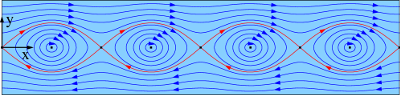
Streamlines of a flow described by the Stuart equation (c = 1.5). On the blue streamlines, the current function has the values ​​-0.8, -0.4,…, 2.4 increasing from the inside to the outside.

Because of this , the streamlines are symmetrical to the x-axis. Between two points with the coordinates (x, -y) and (x, + y), the volume flow disappears regardless of the values ​​of x and y. In other words, just as much fluid flows on the y-axis between (0, y) and the origin from the left half-plane into the right as between the origin and the point (0, -y) from the right half-plane into the left. ${\displaystyle \psi (x,-y)=\psi (x,y)}$

The velocity field is calculated from the derivatives of the current function:

${\displaystyle v_{x}={\frac {\partial \psi }{\partial y}}={\frac {c\sinh(y)}{f(x,y)}}\quad {\text{und}}\quad v_{y}=-{\frac {\partial \psi }{\partial x}}={\frac {{\sqrt {c^{2}-1}}\sin(x)}{f(x,y)}}}$

At the points where the speed disappears, the current function has critical points. These critical locations are at y = 0 and x = ± n π, n = 0,1,2, ... and are marked in the picture with black dots. The current function has the values ​​in the critical points

${\displaystyle \psi (\pm n\pi ,0)=\ln \left(c\cosh(0)+{\sqrt {c^{2}-1}}\cos(\pm n\pi )\right)=\ln \left(c+(-1)^{n}{\sqrt {c^{2}-1}}\right)}$

The value for even is assumed on the red streamlines and the value for odd n only at individual, isolated points in between. The coefficients of the Hessian matrix ${\displaystyle n}$

${\displaystyle \nabla ^{2}\psi ={\begin{pmatrix}{\frac {\partial ^{2}\psi }{\partial x^{2}}}&{\frac {\partial ^{2}\psi }{\partial x\partial y}}\\{\frac {\partial ^{2}\psi }{\partial x\partial y}}&{\frac {\partial ^{2}\psi }{\partial y^{2}}}\end{pmatrix}}}$

are calculated with the current function

${\displaystyle {\begin{aligned}{\frac {\partial ^{2}\psi }{\partial x^{2}}}=&{\frac {1-c^{2}-c{\sqrt {c^{2}-1}}\cos(x)\cosh(y)}{f^{2}(x,y)}}\\{\frac {\partial ^{2}\psi }{\partial x\partial y}}=&{\frac {c{\sqrt {c^{2}-1}}\sin(x)\sinh(y)}{f^{2}(x,y)}}\\{\frac {\partial ^{2}\psi }{\partial y^{2}}}=&{\frac {c^{2}+c{\sqrt {c^{2}-1}}\cos(x)\cosh(y)}{f^{2}(x,y)}}\end{aligned}}}$

The Hessian matrix takes shape in the critical points

${\displaystyle \nabla ^{2}\psi (\pm n\pi ,0)={\begin{pmatrix}{\frac {1-c^{2}-(-1)^{n}c{\sqrt {c^{2}-1}}}{(c+(-1)^{n}{\sqrt {c^{2}-1}})^{2}}}&0\\0&{\frac {c}{c+(-1)^{n}{\sqrt {c^{2}-1}}}}\end{pmatrix}}}$

on. If n is even , the Hessian matrix is

${\displaystyle \nabla ^{2}\psi (\pm n\pi ,0)={\begin{pmatrix}{\frac {1-c^{2}-c{\sqrt {c^{2}-1}}}{(c+{\sqrt {c^{2}-1}})^{2}}}&0\\0&{\frac {c}{c+{\sqrt {c^{2}-1}}}}\end{pmatrix}}}$

indefinite because c> 1 and there is a saddle point . If n is odd , the Hessian matrix is

${\displaystyle \nabla ^{2}\psi (\pm n\pi ,0)={\begin{pmatrix}{\frac {1-c^{2}+c{\sqrt {c^{2}-1}}}{(c-{\sqrt {c^{2}-1}})^{2}}}&0\\0&{\frac {c}{c-{\sqrt {c^{2}-1}}}}\end{pmatrix}}}$

positive definite and there is a minimum. Therefore these points are flown around in a clockwise direction. The positive definiteness results from

${\displaystyle 0<{\frac {1}{c+{\sqrt {c^{2}-1}}}}<1}$ and ${\displaystyle c-{\sqrt {c^{2}-1}}={\frac {1}{c+{\sqrt {c^{2}-1}}}}}$

why

${\displaystyle 0<c-{\sqrt {c^{2}-1}}<1}$ and ${\displaystyle 0<1-(c-{\sqrt {c^{2}-1}})^{2}=2(1-c^{2}+c{\sqrt {c^{2}-1}})}$

See also

Tensoranalysis formula collection

literature

• M. Bestehorn: hydrodynamics and structure formation . Springer, 2006, ISBN 978-3-540-33796-6 , pp. 72 ff .
• Ralf Greve: Continuum Mechanics . Springer, 2003, ISBN 3-540-00760-1 .

Footnotes

1. ↑ Here the product rule with and and the identity is used . ${\displaystyle \operatorname {rot} ({\vec {f}}\times {\vec {g}})=\operatorname {grad} ({\vec {f}})\cdot {\vec {g}}-\operatorname {div} ({\vec {f}}){\vec {g}}+\operatorname {div} ({\vec {g}}){\vec {f}}-\operatorname {grad} ({\vec {g}})\cdot {\vec {f}}}$ ${\displaystyle {\vec {f}}=\operatorname {grad} \psi }$ ${\displaystyle {\vec {g}}={\hat {e}}_{z}}$ ${\displaystyle \operatorname {div} \circ \operatorname {grad} =\Delta }$

Individual evidence

1. ↑ Bestehorn (2006), p. 72
2. ↑ ^{a b} Bestehorn (2006), p. 74f
3. ^ R. Rannacher: Numerical Mathematics 3, Numerics of Problems in Continuum Mechanics. (PDF) Lecture notes for WS 2004/2005. May 16, 2008, p. 132 ff. , Accessed on November 4, 2015 (German).